How to Group Rows in Excel by Name (3 Methods)

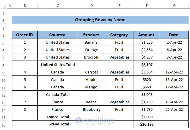
Dataset Overview

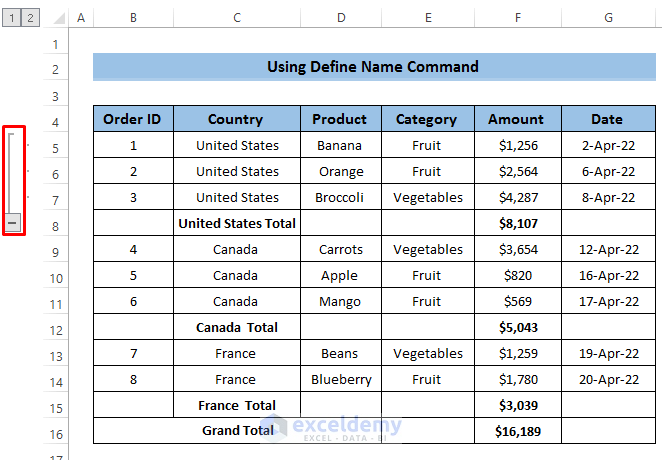
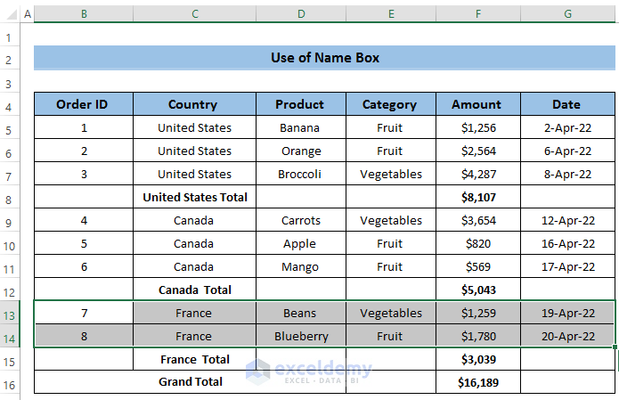
To group rows by name in Excel, follow these three methods using a dataset that includes product, category, and amount information for different countries:

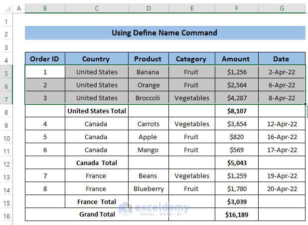
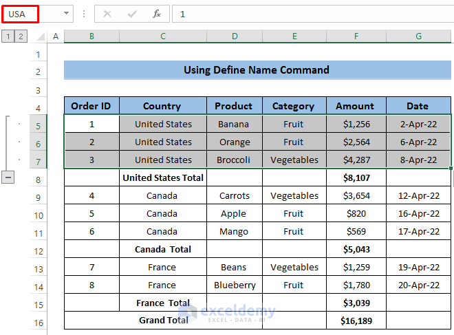
Method 1 – Using the Define Name Command from the Formulas Tab

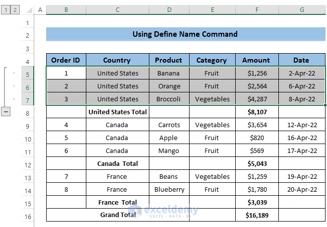
Group Rows:

• Select the range of cells from B5 to G7.

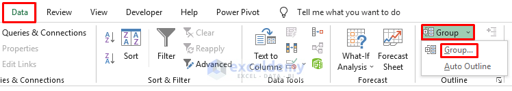
• Go to the Data tab in the ribbon.
• From the Outline group, choose the Group drop-down.
• Select Group from the options.

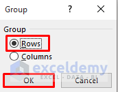
• A Group dialog box will appear; choose Rows and click OK.

• The desired rows are now grouped.
• You can expand or collapse the group using the plus (+) and minus (-) icons.

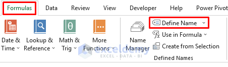
Define a Name:

• Again, select the range of cells from B5 to G7.

• Go to the Formulas tab in the ribbon.
• From the Defined Names group, select Define Name.

• In the New Name dialog box, set your preferred name.
• Click OK.

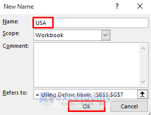
• The group rows will now be named USA in the name box.

Read More: How to Group Rows by Cell Value in Excel

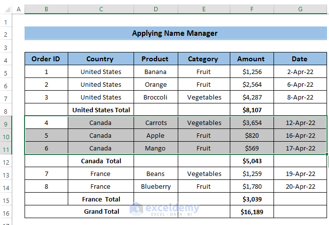
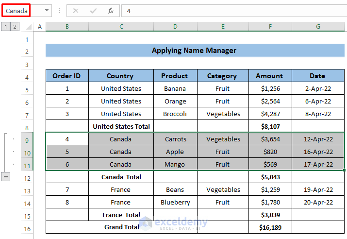
Method 2 – Applying Name Manager to Group Rows by Name

Group Rows:

• Select the range of cells from B9 to G11.

• Go to the Data tab in the ribbon.
• From the Outline group, choose the Group drop-down.
• Select Group from the options.

• A Group dialog box will appear; choose Rows and click OK.

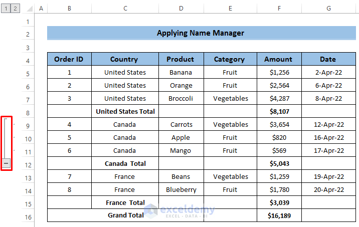
• The desired rows are now grouped.
• You can expand or collapse the group using the plus (+) and minus (-) icons.

Define a Name Using Name Manager:

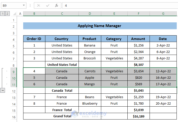
• Again, select the range of cells from B9 to G11.

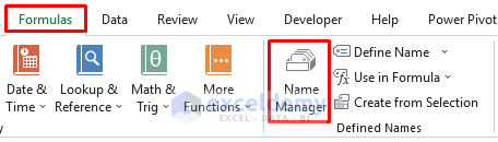
• Go to the Formulas tab in the ribbon.
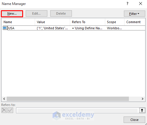
• From the Defined Names group, select Name Manager.

• In the Name Manager dialog box, choose New.

• In the New Name dialog box, set your preferred name.
• Click OK.

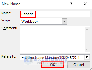
• The group rows will now be named Canada in the name box.

Read More: How to Group and Ungroup Columns or Rows in Excel

Method 3 – Using the Name Box to Group Rows by Name

Group Rows:

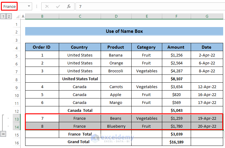
• Select the range of cells from B13 to G14.

• Go to the Data tab in the ribbon.
• From the Outline group, choose the Group drop-down.
• Select Group from the options.

• A Group dialog box will appear; choose Rows and click OK.

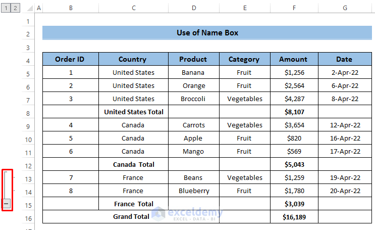
• The desired rows are now grouped.
• You can expand or collapse the group using the plus (+) and minus (-) icons.

Set a Custom Name Using the Name Box:

• Again, select the range of cells from B13 to G14.

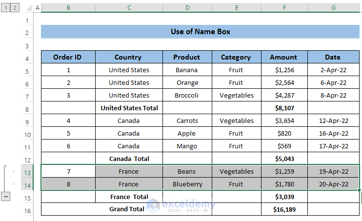
• Look at the name box where cell B13 is displayed.

• Change the name in the box to France according to your dataset.
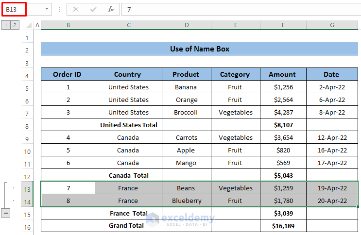
• Press Enter.

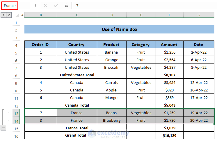
• Now, if you select that group of rows, it will show France in the name box.

Read More: How to Group Rows in Excel with Expand or Collapse

Download Practice Workbook

You can download the practice workbook from here:

Related Articles

• Group Rows with Plus Sign on Top in Excel
• How to Group Rows in Excel
• How to Group Rows with Same Value in Excel
• How to Group Columns Next to Each Other in Excel

<< Go Back to Group Cells in Excel | Outline in Excel | Learn Excel