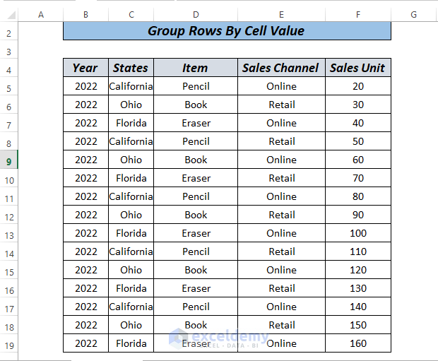
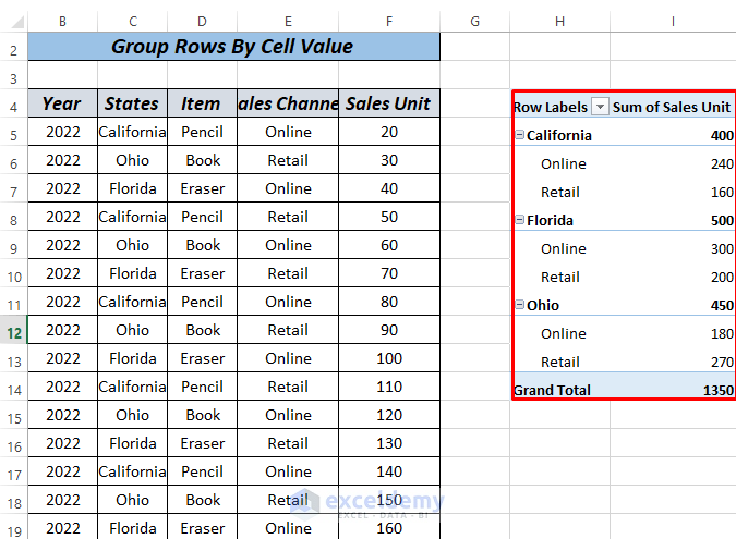
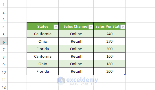
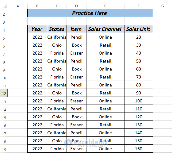
Consider this dataset: Year, States, Items, Sales Channel, and Sales Unit. Let’s say you want to summarize the total units sold at the states and sales channel level, grouped by the States and Sales Channel columns.
Method 1 – Group Rows by Cell Value in Excel Using DataTab
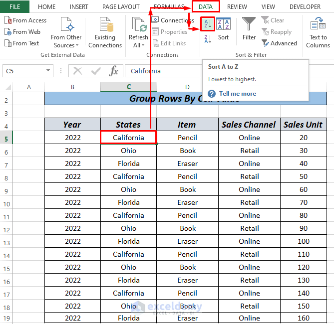
- Select one of the cells in the States column.
- Go to the Data tab and select Ascending sorting (Sort A to Z).
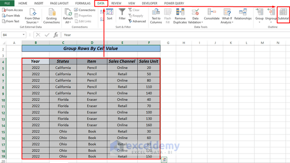
 Select the entire table.
- Go to the Data tab and select Subtotal.
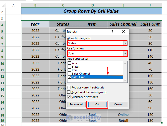
 In the pop-up window, select “States,” “Sum,” and check “Sales Unit,” respectively.
- Press OK.
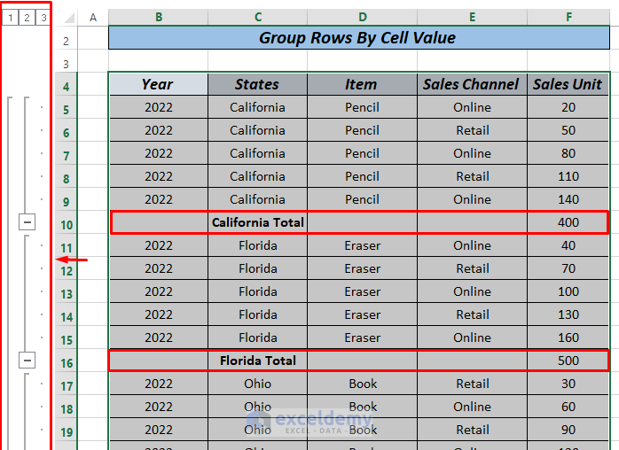
 The worksheet will look like the following image, gaining new rows for sums.
Read More: How to Group Rows in Excel
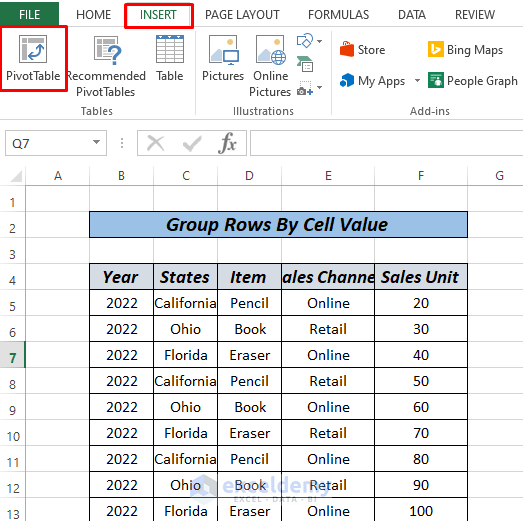
Method 2 – Group Rows by Cell Value by Pivot Table
- Go to the Insert tab and click on Pivot table.
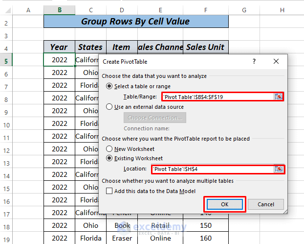
 A dialogue box will pop up. Select the table range and select a cell where the table will be.
- Click on OK.
 We will get another dialogue box. Check and drag the States and Sales Channel to the Row and Sales Unit in the Values section.
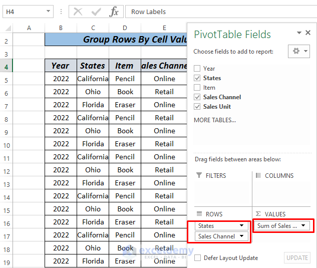 Excel will print the table.
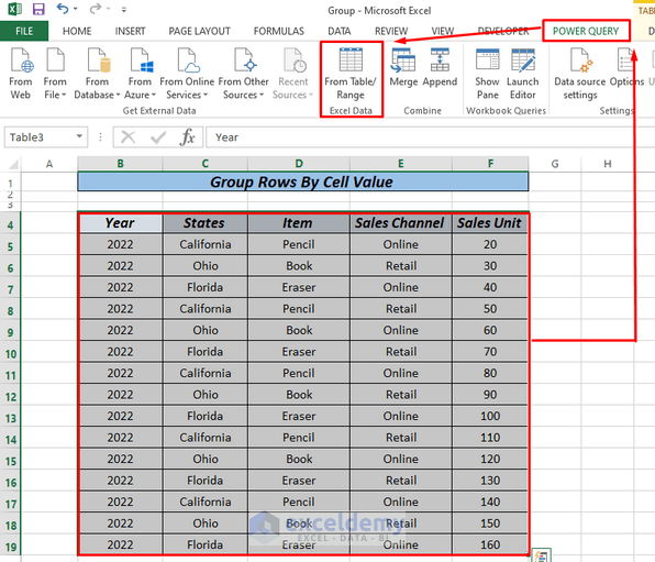
Method 3 – Group Rows by Cell Value Using Power Query
- Select the entire table.
- Go to the Power Query tab and click From Table/Range. If you don’t have the tab, go to Data, then From Table/Range in the Get Data section. You may need to confirm the table selection.
 A new window will pop up and we will select Group By from the Home tab.
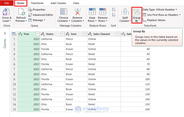 A dialogue box will pop up and we will select Advance and fill the boxes as per the image shown. Click OK.
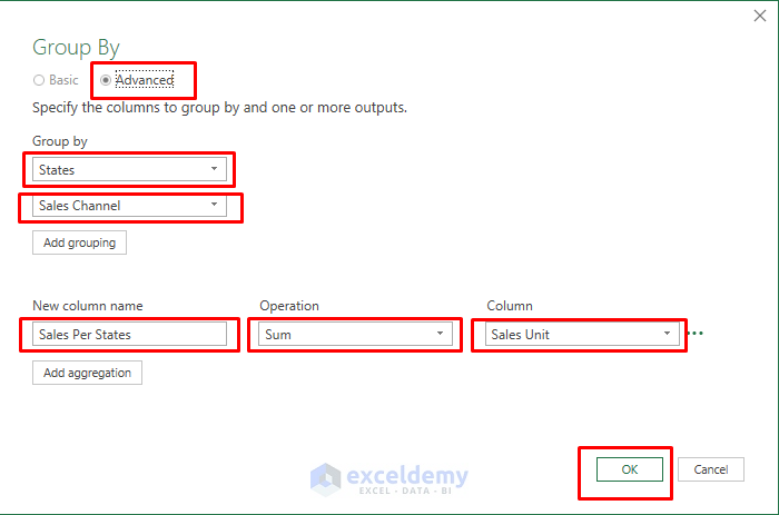 Click on the Close & Load option and the table will automatically be generated in the original workbook.
Practice Section
We’ve attached a practice workbook where you can practice these methods.
Download Practice Workbook
Related Articles
- How to Group Rows in Excel by Name
- Group Rows with Plus Sign on Top in Excel
- How to Group Columns Next to Each Other in Excel
- How to Group Rows with Same Value in Excel
- How to Group Rows in Excel with Expand or Collapse
<< Go Back to Group Cells in Excel | Outline in Excel | Learn Excel
Get FREE Advanced Excel Exercises with Solutions!
