How to Insert Subtotals in Excel (7 Unique Methods)

When dealing with extensive datasets, it becomes crucial to summarize and organize information effectively. This is where the power of subtotals comes into play. This tutorial will give you a complete overview of how to insert subtotals in Excel with proper illustrations.

Subtotals allow you to break down data into manageable groups, calculate aggregate values, and gain a deeper understanding of your information. Today we’ll try to cover everything you need to know, from preparing your data to customizing subtotals based on your requirements.

Basics of Subtotals

In generic terms, subtotal refers to the total of one set of a larger group of collections. For example, suppose you got 100 marks in your last semester, where the marks of the math course were obtained from the three class tests that you had. In the first class test, you got 10, in the second you got 15, and in the last class test, you got 20. So now you want to know only your math score out of 100 marks. To get that quickly, you can use subtotal.

Subtotals in Excel are a way to calculate summary statistics for groups or subsets of data within a larger dataset. They allow you to create subtotals based on a specified column or columns and perform calculations such as SUM, AVERAGE, MAX, MIN, COUNT, Product, etc.

How to Insert Subtotals in Excel: 7 Unique Methods

This section will cover 7 unique approaches to grouping your data and adding subtotals to it. With real-life and practical datasets, we will try to create a visualization of how to insert subtotals in Excel worksheet.

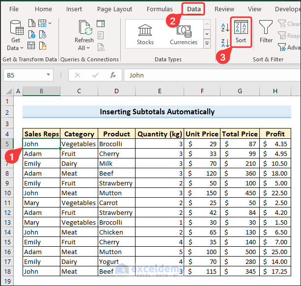
1. Insert Subtotals in Excel Automatically

Suppose we have a dataset of seller information where sales reps sold different categories of products. The dataset includes the quantity of sold items, unit price, total price, and profit gained from selling those products. Using this dataset, we will find subtotals and grand totals in Excel.

We will use the Subtotal feature of Excel to insert subtotals automatically. For this:

• Select a random cell > go to the Data tab > click Sort.

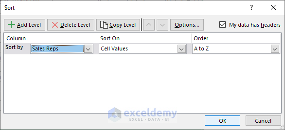
• The Sort dialog box will pop up on the window.
• In the Sort by field, select the column on the basis of which you want to insert subtotals.
• Keep Cell Values in the Sort On field.
• Order will be ascending: A to Z.
• Click OK.

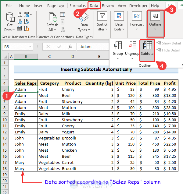
• This will sort the Sales Reps column alphabetically.

Now we will use the built-in feature which is also known as the subtotal shortcut in Excel

• Again click on a cell in the range > select Subtotal under Outline group from the Data tab.

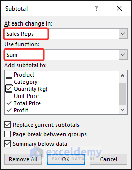
• The Subtotal dialog box will appear now. We will insert subtotals in Excel using the SUM function.
• At each change in field should hold the data on which you will insert subtotals.
• Put the SUM function in the Use function field as we want to calculate the total value.
• Click OK.

Now you will be able to insert subtotals in Excel. The sales Reps column will hold subtotals and grand totals.

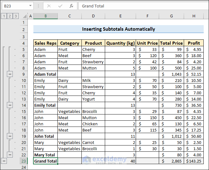
• The icon at the top left corner with numbers 1, 2, and 3 will command you how to use subtotals in Excel. It allows handling the groups and showing and hiding subtotals in Excel.

Read More: How to Sort Subtotals in Excel

2. Add Multiple Subtotals

The previous method allows you to add a single subtotal. However, the subtotal feature also allows you to add multiple subtotals in Excel. You can insert multiple subtotals both in the same column or in different columns.

2.1. Insert Multiple Subtotals in Different Columns

In the previous section, we have already shown how we can apply subtotal upon the Sales Reps column. So, in this section, we will add another subtotal based on Category.

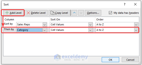
• Open the Sort dialog box from the Data tab.
• First Sort by Sales Reps.
• Add another level.
• Firstly we have sorted by Sales Reps, now we will sort by Category.
• Click OK.

• Open the Subtotal dialog box from the Data tab as described in Method-1.
• Choose Sales Reps in the At each change in field.

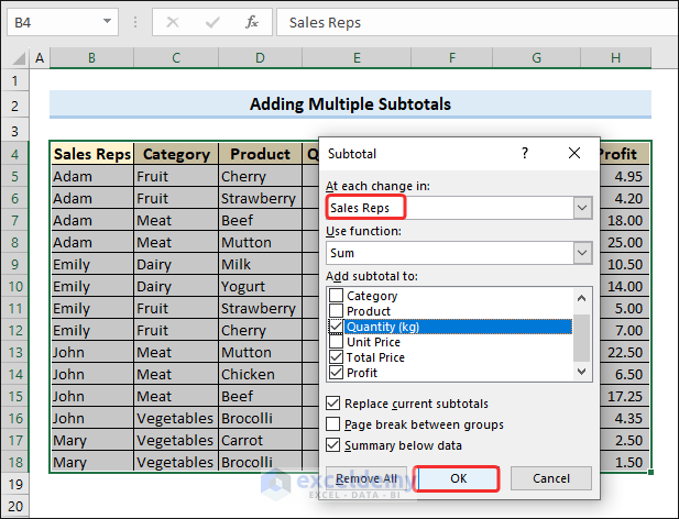
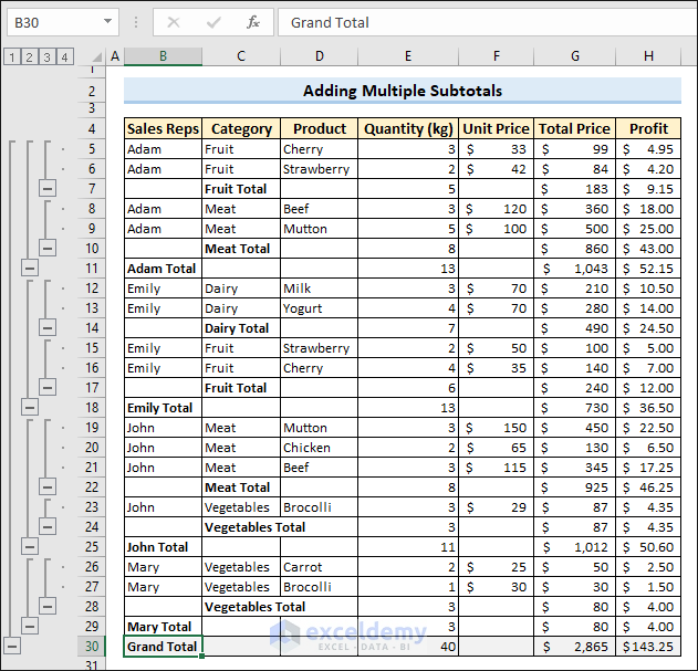
• Excel will insert Subtotals to the Sales Reps column.
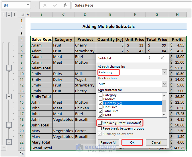
• Again open the Subtotal pop-up.
• This time ensures each change in Category.
• Make sure the Replace Current Subtotals field is unmarked. If not, it will clear the previous subtotal and result in a single subtotal.
• Click OK.

Now we will be able to group multiple times and insert subtotal in Excel.

Select another change in the Subtotal box if you want to add subtotals further.

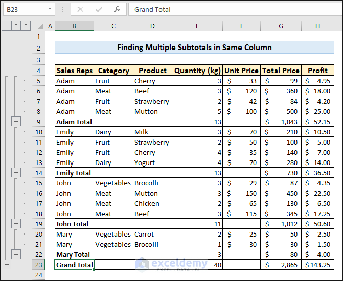
2.2. Find Multiple Subtotals in Same Column

Now, we will insert multiple subtotals in the same column. We will calculate the average and standard deviation after calculating the total. So, you will need two more functions. First, we will choose the AVERAGE function and then the StdDev function.

We will start from after inserting subtotals to Sales Reps (gained from Method-1) using the SUM function.

• After that, open the Subtotal box 2 times more.
• First time, choose the AVERAGE function and second time select the StdDev function.

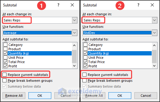
• The AVERAGE function will find out the average of the selected columns.
• The StdDev function will calculate the standard deviation.

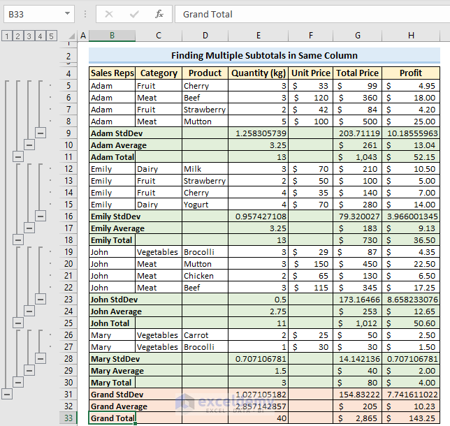
Based on each of these functions, subtotals will be inserted into your data.

3. Insert Subtotals in Excel Table

You can’t apply subtotals directly in the Excel table. The Subtotal feature won’t work here.

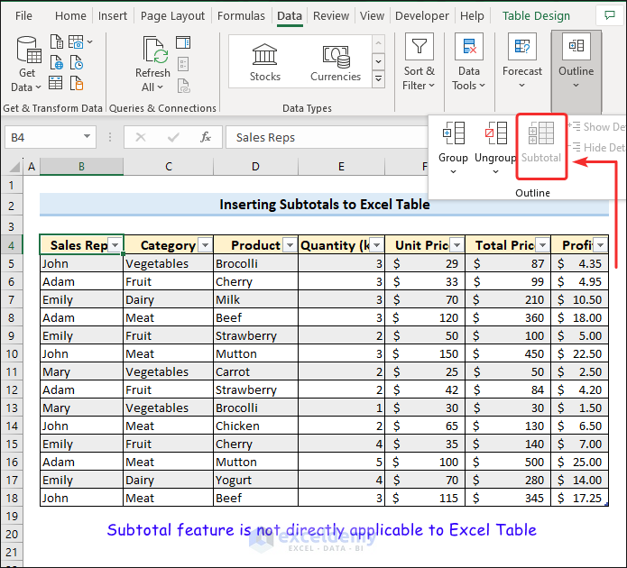
If you want to insert subtotals, you have to convert the table to range first.

• Select a random cell in your table and go to the Table Design tab > select Convert to Range under the Tools group.

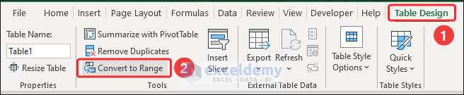
• Microsoft Excel will ask you whether you want to convert the table to a range. Confirm it by clicking Yes.

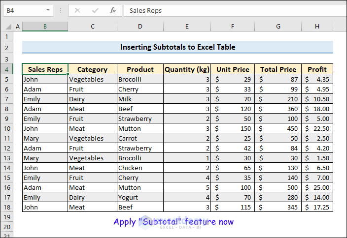
Excel will now convert the table to a normal range. You can now apply the subtotal feature to insert subtotals.

4. Apply SUBTOTAL formula in Excel with Filter

Till now we have used the Subtotal feature. Excel also has the SUBTOTAL function available to add subtotals to your data. We will use the function for filtered data.

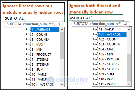
The syntax of the SUBTOTAL function:

Here, the first argument: function_num is described by some numbers (1-9 and 101-109) denoting different functions.

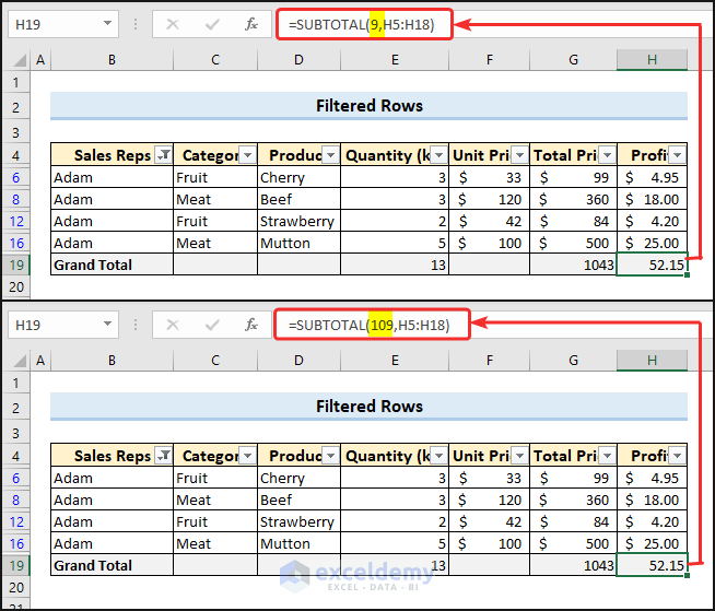
4.1. Subtotals in Filtered Out Rows

We have applied the following SUBTOTAL formula to insert subtotals.

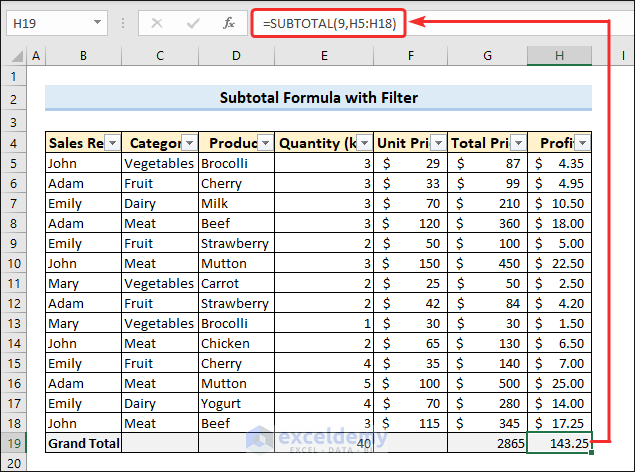
As we used the first argument: 9, it will ignore the filtered cell

• Click the drop-down arrow at the Sales Reps column and choose a name (i.e. Adam) to filter by that name.

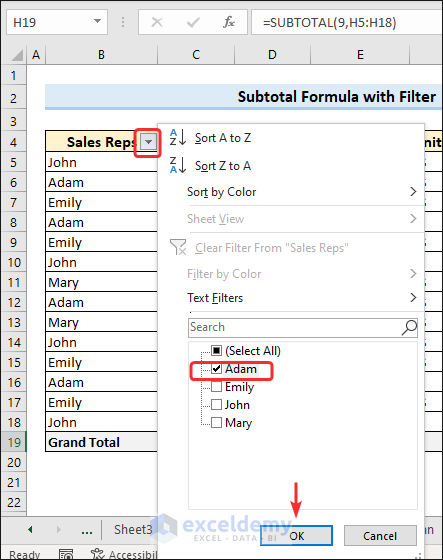
You will observe the function to calculate subtotals only for the filtered cells, it will ignore the rest.

The image below demonstrates the output of the SUBTOTAL function for both arguments 9 and 109.

Read more: How to Use SUBTOTAL in Excel with Filters

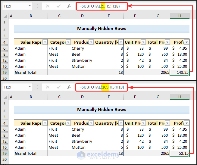
4.2. Subtotals in Manually Hidden Rows

If you want to see the output of the SUBTOTAL function for manually hidden rows, then hide rows by right-clicking on the row number and choosing Hide from the context menu.

Then compare the output for arguments 9 and 109. Argument 9 will include the cells of manually hidden rows but argument 109 will ignore them.

5. Find Subtotals with VBA Code

You can customize a VBA code for your dataset and insert subtotals to your data by using VBA macro. You will need to launch the VBA editor for that. Let’s follow the instructions to use the VBA code for subtotal in Excel!

• Press ALT+F11 to launch the Visual Basic Editor window.
• Click Insert on the Toolbar > select Module.

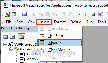
• Insert your VBA code on the Module window.

Code:

Sub Calculate_Subtotal()
Dim iColumn As Integer
Dim iValue As Integer
Dim xValue As Integer
Application.ScreenUpdating = False
iValue = 5
xValue = iValue
Range("B5").CurrentRegion.Offset(1).Sort Range("B6"), 1
Do While Range("B" & iValue) <> ""
    If Range("B" & iValue) <> Range("B" & (iValue + 1)) Then
    Rows(iValue + 1).Insert
    Range("B" & (iValue + 1)) = "Subtotal " & Range("B" & iValue).Value
    For iColumn = 7 To 8 'Columns to Calculate Sum
    Cells(iValue + 1, iColumn).Formula = "=SUM(R" & xValue & "C:R" & iValue & "C)"
    Next iColumn
    Range(Cells(iValue + 1, 1), Cells(iValue + 1, 8)).Font.Bold = True
    iValue = iValue + 2
    xValue = iValue
    Else
    iValue = iValue + 1
    End If
    Loop
Application.ScreenUpdating = True
End Sub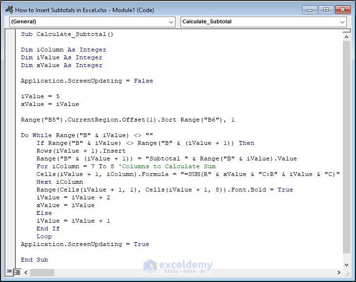

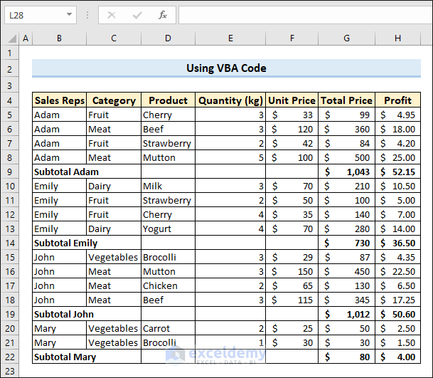
• Click the Run button to execute the VBA code.

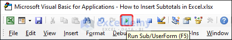
Excel will now insert subtotals in your data based on Sales Reps.

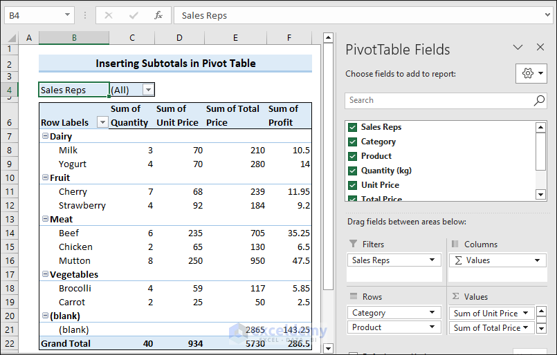
6. Add Subtotals in Excel Pivot Table

Let’s say we have a Pivot Table in our Excel sheet and we want to add subtotals to the grouped data in the Pivot Table. A Pivot Table is used to categorize large datasets according to criteria.

There are four fields in the Pivot table and we have formatted pivot table using our data in those fields:
1. Filter: Sales Reps

2. Columns: Blank
3. Rows: Category, Product
4. Values: Quantity, Unit Price, Total Price, and Profit

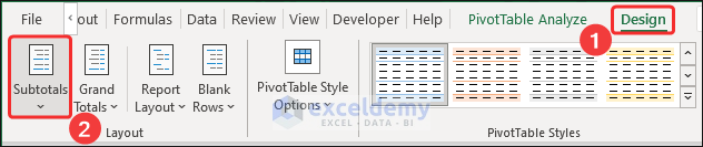
• Go to the Design tab > click the dropdown of Subtotals option under Layout group.

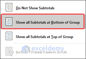
• Select Show all Subtotals at Bottom of Group from the dropdown menu.

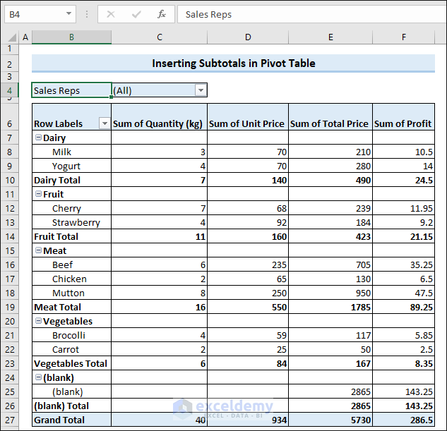
The pivot table will now insert subtotals at the bottom of each group based on Row Labels. Excel will also add the grand total of the group at the bottom of the table.

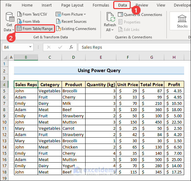
7. Use Power Query to Insert Subtotals

Power Query is a powerful data transformation and data preparation tool that is part of Microsoft Excel and Power BI. It allows you to import, transform, and combine data from various sources into a format that is suitable for analysis and reporting.

In this section, we will use a power query to insert subtotals for groups.

• Click a cell in the range > go to the Data tab > click From Table/Range under Get & Transform Data.

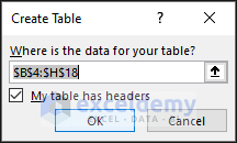
• Click OK on the Create Table dialog box.

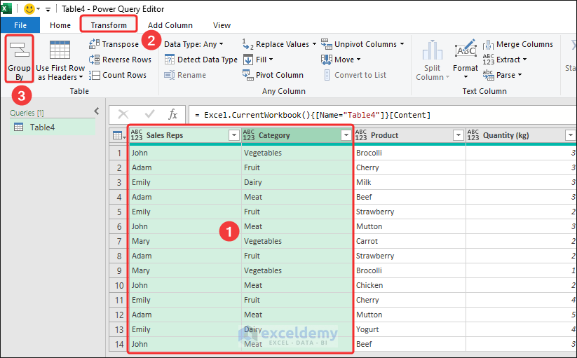
• Excel will shift you to the Power Query Editor window.
• Select the columns (i.e., Sales Reps and Category) in the data that you want to deal with > click Group By icon from the Transform tab.

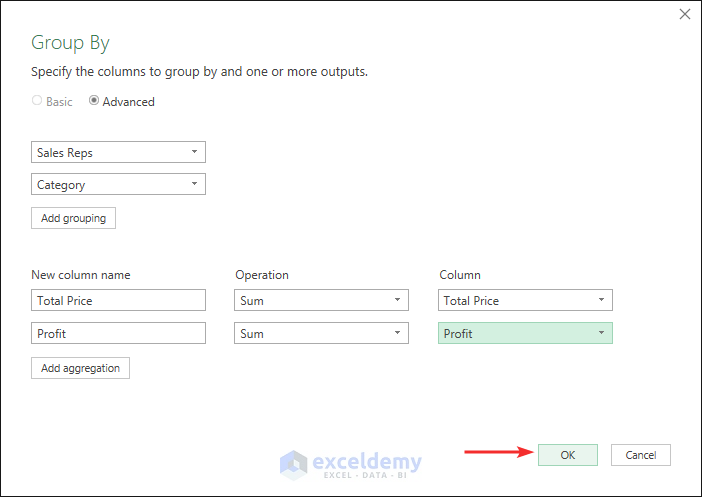
• In the Group By dialog box, give a New column name.
• Select the type of operation that you want to perform (i.e., SUM).
• Select the Column where you want to perform the calculation (i.e., Total Price).
• Click on Add Aggression to group further.

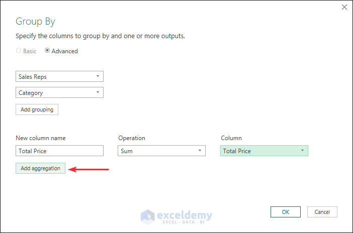
• To calculate subtotals of the Profit, choose Profit in the Column field and Sum in the Operation field. Give this aggression a name (i.e., Profit).
• Click OK.

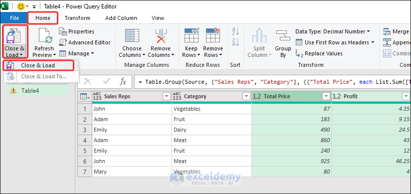
• You will see subtotals inserted based on the Sales Reps and Category.
• Go to the Home tab > click dropdown of Close & Load > select Close & Load.

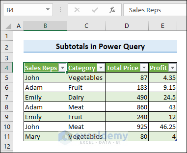
The Power Query editor will load your grouped data with subtotals to the Excel worksheet.

How to Remove Subtotals in Excel

If want to remove subtotals from the range, you have to utilize the Subtotal feature again.

• Open the Subtotals dialog box from the Data tab > click Remove all.

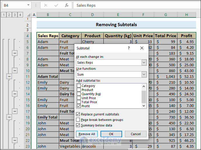
• You will get your data converted to the normal range by removing groups and subtotals from it.

Frequently Asked Questions

1. Why Can’t I remove subtotals in Excel?

Subtotals may not work for several reasons.

i) Protected worksheet: You will need to unprotect your sheet if it is protected with a password.

ii) Shared workbook: You may need to unshare the workbook or check with the workbook if the workbook is shared among multiple users

iii) Custom formulas or macros: If subtotals were added using custom formulas or macros, you may need to modify or delete the formulas/macros to remove the subtotals.

2. How do I collapse or expand subtotals in Excel?

To collapse or expand subtotals in Excel, you can use the grouped outline feature. Excel automatically adds outlining symbols that allow you to collapse or expand the subtotal groups. Clicking on the minus (-) or plus (+) symbols next to the group rows will collapse or expand the subtotals, respectively.

3. Can I automatically update subtotals in Excel when the data changes?

Yes, you can set Excel to automatically update the subtotals when the data changes. You can also refresh the subtotals manually by right-clicking on a subtotal row and choosing “Refresh” from the context menu. If it is not automatically updated, ensure your workbook auto calculate formulas.

4. Is AGGREGATE the same as SUBTOTAL function in Excel?

No, there are differences between AGGREGATE and SUBTOTAL functions although the syntax is similar.

Key Takeaways from the Article

• The “Subtotal” feature in Excel allows you to insert subtotals for groups of data based on specified columns.
• To insert subtotals, select the range of data and go to the “Data” tab, then click on the “Subtotal” button in the “Outline” group.
• You can add multiple levels of subtotals by selecting multiple columns to subtotal by.
• Subtotals can be collapsed or expanded using the grouped outline feature, indicated by minus (-) and plus (+) symbols.
• Subtotals can be automatically updated when the data changes by using Excel’s tables or dynamic named ranges.

Download Practice Workbook

You can download the practice workbook from here.

Conclusion

So, we have learned how to insert subtotals in Excel using some convenient ways. It enables you to apply functions like Sum, Average, Count, and more to aggregate and summarize data depending on chosen columns. Subtotals can be added at different levels, and you can change how they look to suit your tastes. For improved data organization, you can collapse or enlarge subtotals using the grouped outline function. When the underlying data changes, subtotals can be updated automatically, guaranteeing precision and effectiveness. Additionally, you can use subtotals with pivot tables or charts by exporting or copying them to other programs. You may efficiently evaluate and present compiled data in your Excel worksheets by making use of these features.