How to Group Rows in Excel – 5 Easy Methods

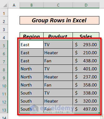
The dataset showcases data of a company that operates in 3 regions and sells 3 different products- TV, Heater, and Fan.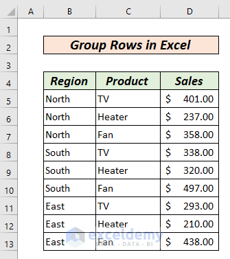

Method 1 – Grouping Rows Using the Group Feature

• Go to the Data tab and click Group.

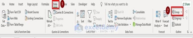
• In the dialog box, select Rows.
• Press OK.

Rows will be grouped.

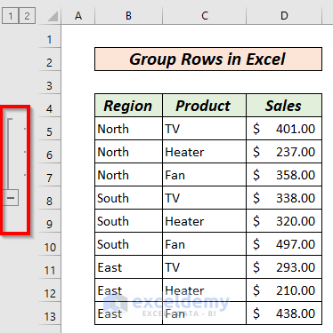
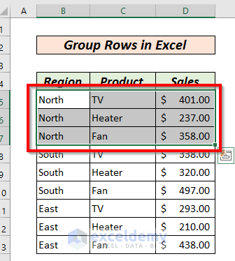
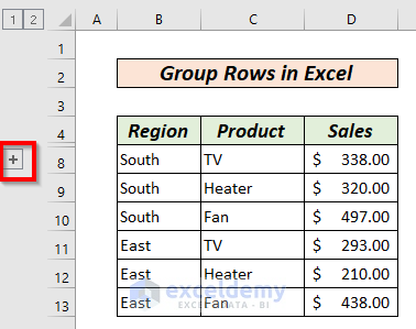
Rows 5, 6, 7 are grouped. Use the minimize symbol (-) to collapse the rows.

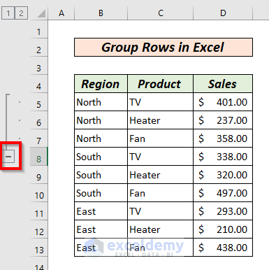
A plus sign(+) will be displayed. Click it to expand the grouped rows.

Read More: How to Group Rows in Excel with Expand or Collapse

Method 2 – Creating Nested Groups to Group Different Rows

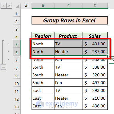
To group TV and Heater sold in the North Region region:

• Go to the Data tab >> Group.
• Select Rows in the dialog box.
• Click OK.

This is the output.

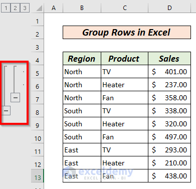
Rows 5, 6, 7 form the outer group and rows 5 and 6 form the inner group.

Read More: How to Group Rows by Cell Value in Excel

Method 3 – Grouping Rows Using the SHIFT + ALT + Right Arrow Key

• Select the rows you want to group.

• Press SHIFT + ALT + Right Arrow Key ().
• In the dialog box, select rows.
• Click OK.

The selected rows are grouped.

Use the minimize symbol (-) to collapse the rows.

Click the  plus sign(+) the plus sign to expand the group.

Method 4 – Grouping Rows in Excel Using the Auto Outline

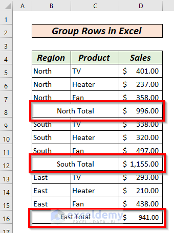
An additional regional total row was inserted.

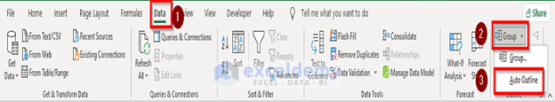
• Go to the Data tab >> Group >> Auto Outline.

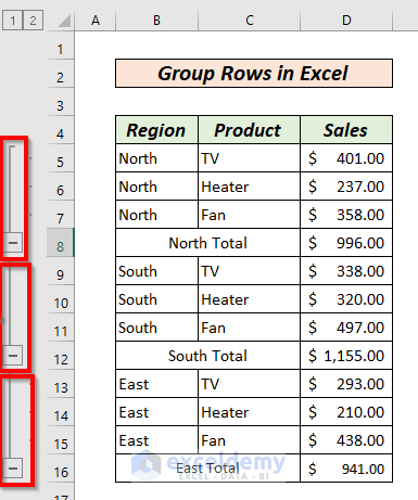
Data will be grouped according to the different regions.

Method 5 – Grouping Rows in Excel Using the Subtotal Feature

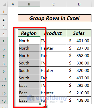
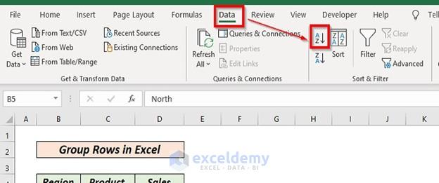
• Select the Region column.
• Go to the Data tab and select Sort A to Z (Lowest to Highest).

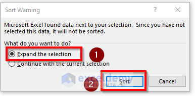
• In the dialog box, select Expand the selection and click Sort.

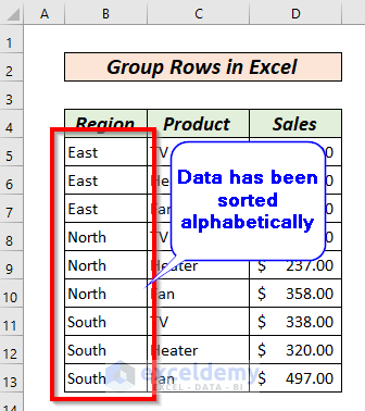
This is the output.

• Select the entire data range.

• Go to Data  >> select Subtotal.

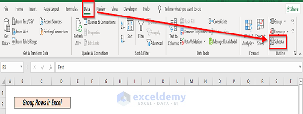
A new dialog box will open.

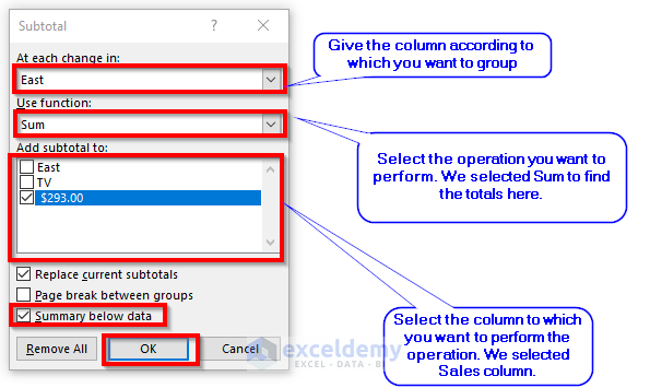In the dialog box:

• In At each change in:, select the data of the column in which you want to group rows.
• In Use function:, add a function. Here, SUM.
• In Add subtotal to:, select the column in which the mathematical operation will be performed.
• Check Summary below data.
• Click OK.

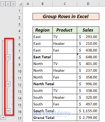
Data will be grouped.

Read More: How to Group Rows in Excel by Name

Practice Section

Practice here.

Download Practice Workbook

Related Articles

• How to Group Rows with Same Value in Excel
• Group Rows with Plus Sign on Top in Excel
• How to Group Columns Next to Each Other in Excel

<< Go Back to Group Cells in Excel | Outline in Excel | Learn Excel