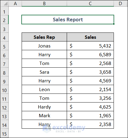
Example 1 – Consolidating Data from Multiple Rows
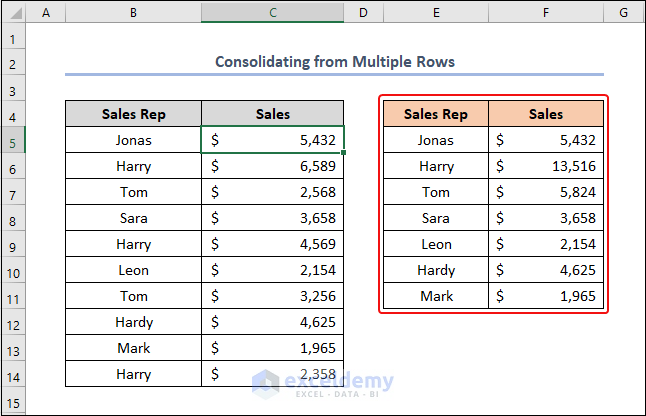
There are repeated names in the dataset:
To consolidate repeated Sales Reps accounts in a single row:
Steps:
- Select E4.
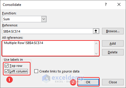
- Go to the Data tab and select Consolidate.
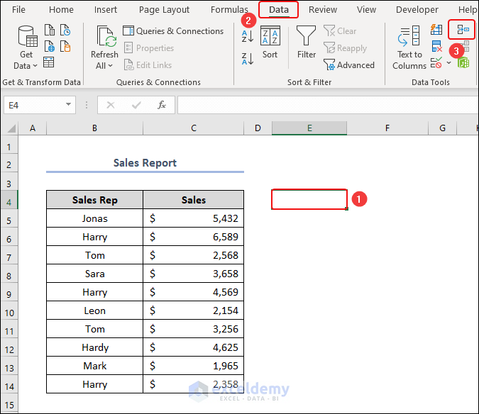
- In Consolidate, click the Reference box.
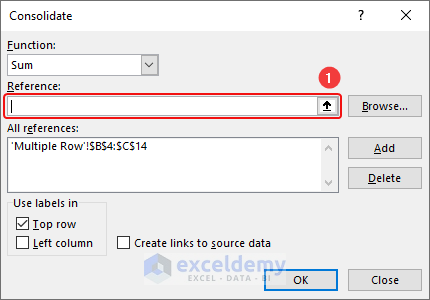
- Select B4:C14.
The selected cell reference is displayed both in Reference and All references.
- Check Top Row and Left Column.
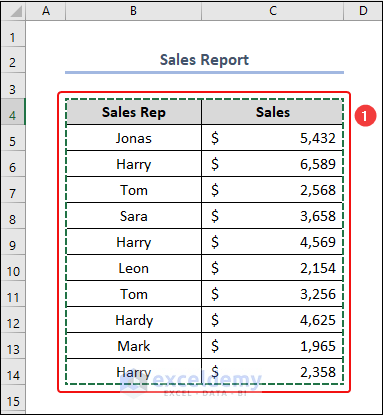
This is the output.
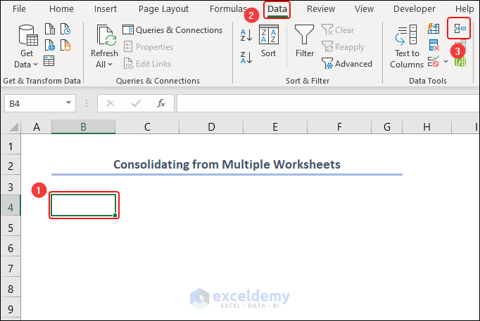
Example 2 – Consolidating Data from Multiple Worksheets
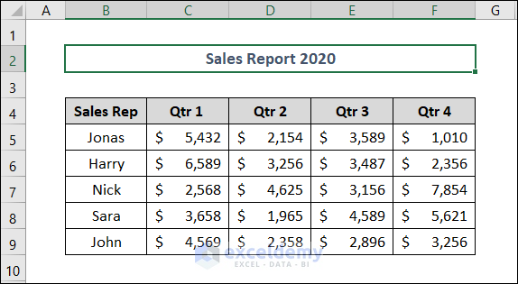
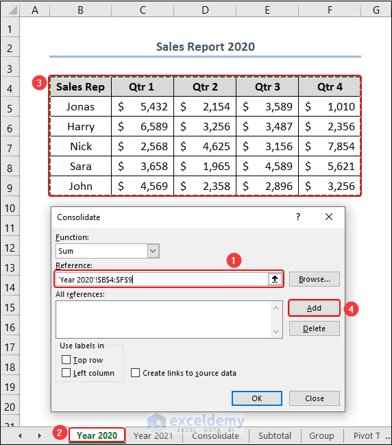
You have Sales Reports in two different worksheets:
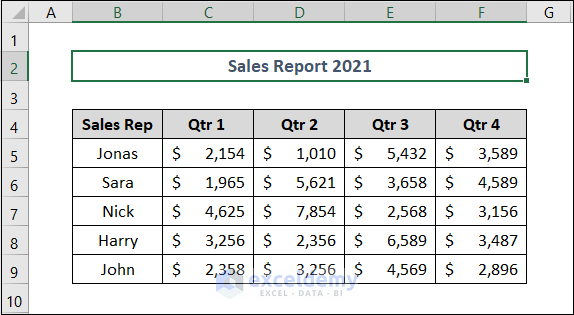
In the 2021 Sales Report, the names of Sales Reps are in a different order.
Steps:
- Open a new worksheet: Consolidate and select B4.
- Go to the Data tab and select Consolidate.
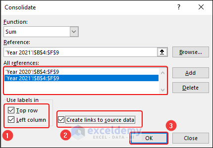
- In Consolidate, click the Reference box.
- Go to the worksheet Year 2020 and select B4:F9.
- Click Add.
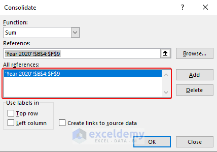
The selected cell references are displayed in All references.
- Select the cell range in the Year 2021 worksheet and click Add.
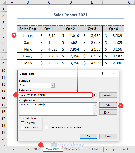
The cell references of the two sheets are displayed in All references.
- Check the 3 boxes marked below.
- Click OK.
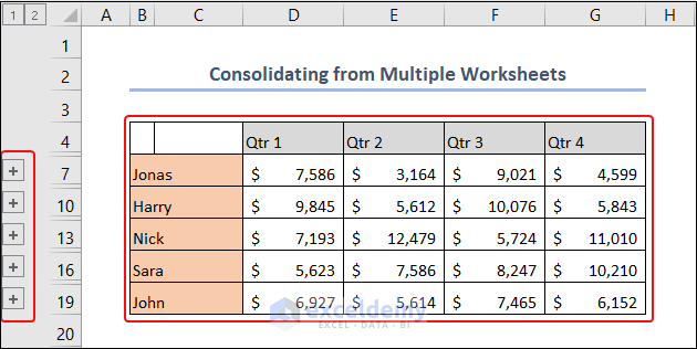
- The ( + ) sign is displayed on the left side of the spreadsheet. Click to see the yearly sales individually.
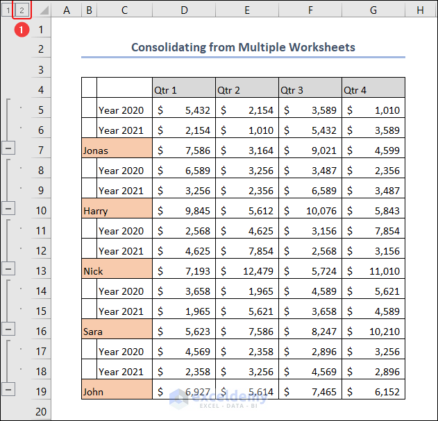
- Click 2 to expand the dataset.
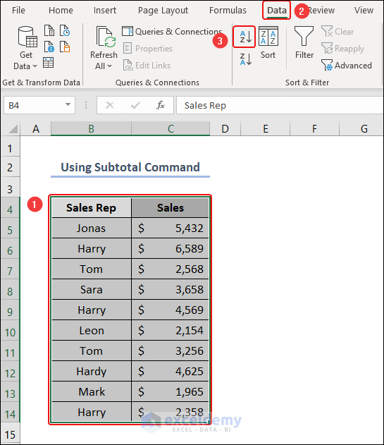
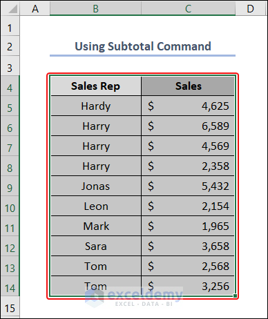
Example 3 – Using the Subtotal Command to Group Data in Excel
Steps:
- Select B4:C14.
- Go to the Data tab and select Sort A to Z in Sort & Filter.
Data is displayed in alphabetical order.
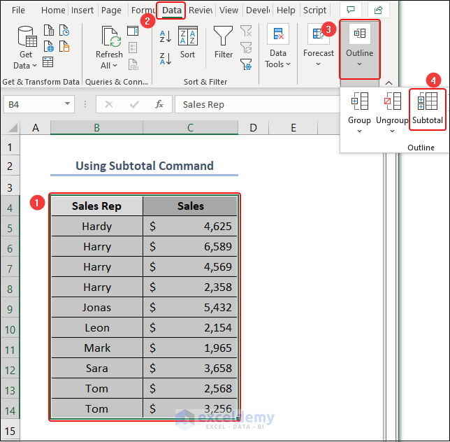
- Go to the Data tab and select Outline.
- Choose Subtotal.
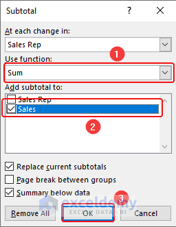
- Select the options marked in the image below and click OK.
The dataset is grouped and ( – ) signs are displayed (rows and columns are expanded).
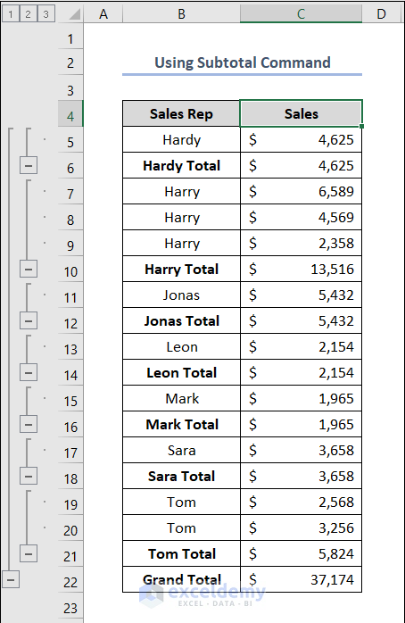
- Click 2 to see individual Totals:
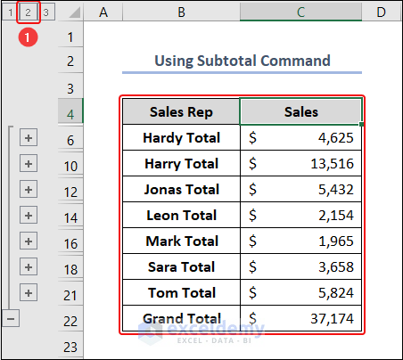
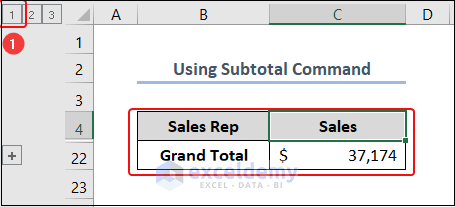
- Click 1 to see the Grand Total.
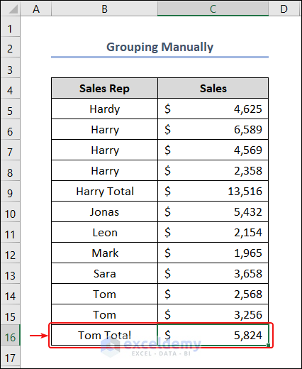
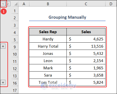
Example 4 – Using Manual Grouping in Excel
Steps:
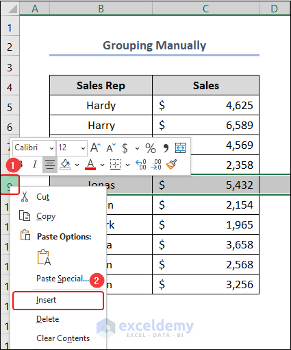
- Right-click row 9.
- Choose Insert.
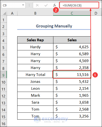
- A new row is created. Here, Harry Total in B9.
- Enter the formula below in C9.
=SUM(C6:C8)
- Follow the same steps for row 16.
- Select B6:C8.
- Go to the Data tab and select Outline.
- Choose Group.
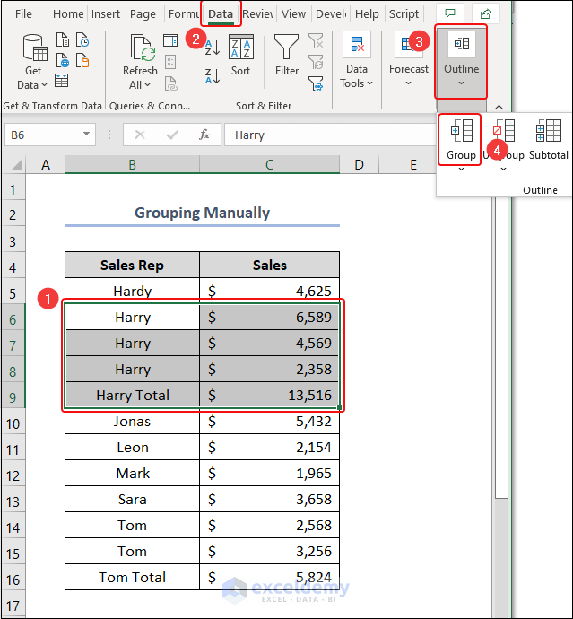
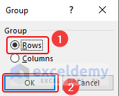
- In Group, select Rows.
- Click OK.
- Group the rows of Tom’s account.
The dataset is grouped.
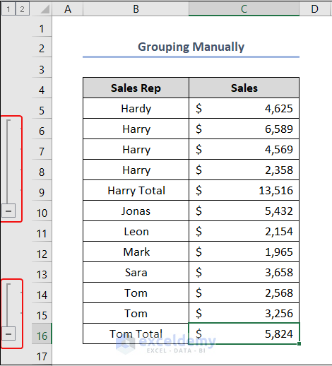
- Click 1 to collapse the dataset.
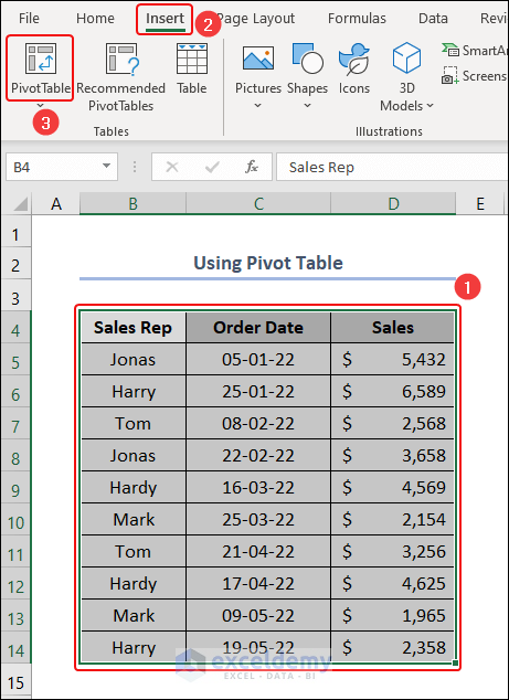
Example 5 – Inserting a Pivot Table
Steps:
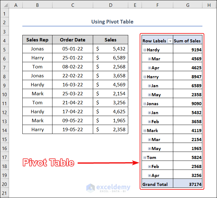
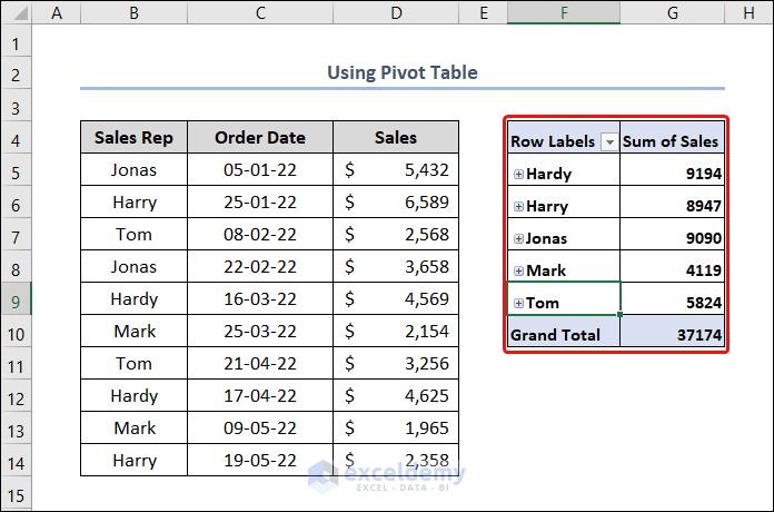
- Select B4:D14.
- Go to the Insert tab and select PivotTable.
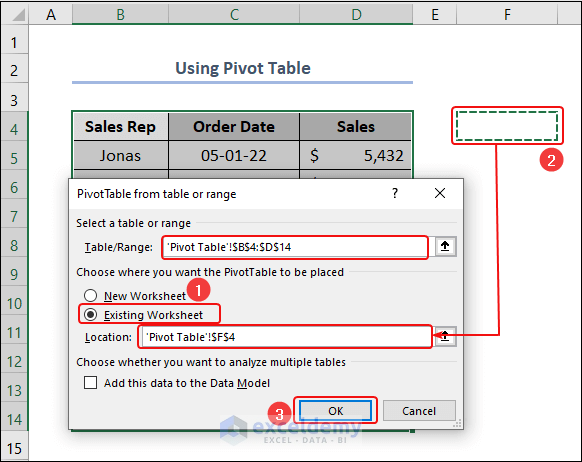
- In PivotTable from table or range, select Existing Worksheet.
- Click the Location box and select F4.
- Click OK.
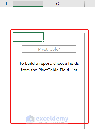
The pivot table is displayed:
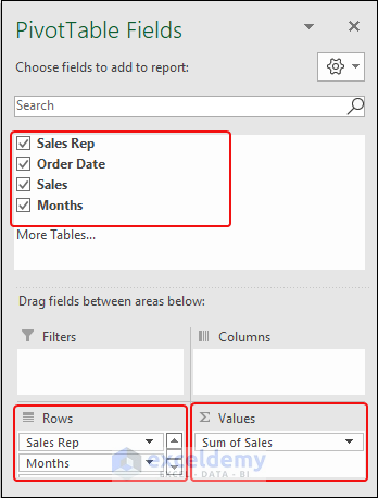
- In PivotTable Fields, drag the fields as shown in the image below.
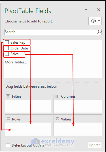
Rows contain Sales Rep and Months. Values contain Sum of Sales.
This is the output.
- Click ( – ) to collapse the table.
Download Practice Workbook
Download the following Excel workbook.
<< Go Back To Consolidation in Excel | Merge Sheets in Excel | Merge in Excel | Learn Excel
Get FREE Advanced Excel Exercises with Solutions!

Nice writing. Can I ask a ques? We are a small merchandise startup. In recent time, we,re maintaining some sheets. In one of them, we are storing the monthly sales of different products ( as example: different designs of t’s). But i wanna group them. Like, product with sales greater than 2000$ is small,>2000 but 5000 is key product. So, we can concentrate on the best seller. Help me in this.thanks.
Hello LINCHEN NUMBY,
Thanks for your comment. Here, we’re very eager to help this kind of new startup.
For ease of understanding, you may download the workbook to go along with the approach.
From your comment above, we’ve made an imaginary dataset for your company. Let’s have a look at this first.
Then, construct a new column named Group under Column E.
After that, select cell E5 and enter the following formula.
=IF(D5>5000,"Key Product",IF(D5>=2000,"Large",IF(D5<2000,"Small")))Following this, press ENTER.
Now, bring the cursor to the right-bottom corner of cell E5; instantly, it’ll look like a plus (+) sign. Basically, it’s the Fill Handle tool.
Currently, double-click on it to get results in the following cells also.
Finally, the results are here.
Alternatively, you can use the following formula instead of the previous one.
=IFS(D5>5000,"Key Product",D5>2000,"Large",D5<2000,"Small")So, that’s all from me on this problem. Feel free to contact us for other inquiries. Follow our website Exceldemy to explore more about Excel.