How to Do Consolidation in Excel (2 Useful Cases)

Looking for ways to consolidate data in Excel? Then, this is the right place for you. Sometimes, we need to consolidate data to summarize the data from separate ranges into a single output range. With this in mind, this article hopes to guide you on how to do consolidation in Excel.

Download Practice Workbook

You can download the practice workbook from the link below.

Introduction of Consolidate Feature in Excel

Data consolidation is the process of integrating different parts of the information into a single, structured format. In fact, you can merge rows, columns, and separate worksheets using the built-in consolidation feature in Excel.

Now, to perform data consolidation, go to Data > Consolidate options in the Data Tools section.

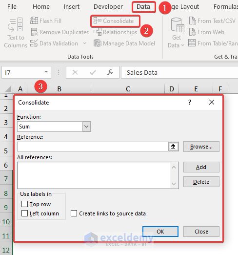
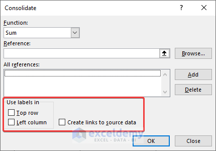
Now, let’s learn about the various options of the Consolidate dialog box.

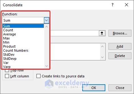
• Firstly, you can use the Function drop-down to perform various mathematical operations.

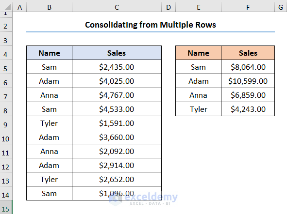
In this example, the Sum function adds up the Sales amount for each employee.

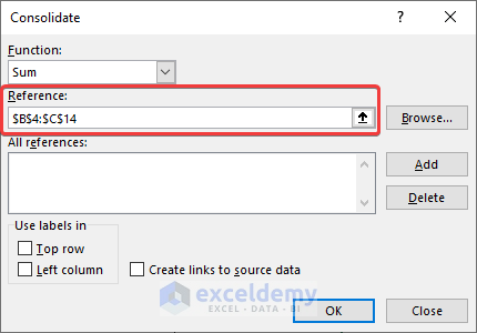
• Secondly, the Reference box allows us to select the dataset from other worksheets

Here, the $B$4:$C$14 cells represent the chosen dataset.

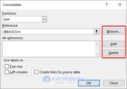
• Moreover, you can use the Browse option to select data from a separate workbook.
• Following, the Add and the Delete options allow you to select multiple datasets or remove a dataset.

• Thirdly, the Top row and Left column options recognize the position of the table headers.
• Lastly, the Create links to source data option link the original data with the consolidated report.

2 Cases to Do Consolidation in Excel 

We’ll show 2 different cases to perform data consolidation using the Consolidate feature. So, without further delay, let’s see the process step-by-step.

1. Consolidation of Data from a Range of Cells

Our, first case considers the scenario where you have a range of cells in your dataset.

Let’s consider the following dataset shown in B4:C14 cells. Here, the columns show the Employee Names, and their corresponding Sales in USD.

1.1 Consolidation of Multiple Rows

Clearly, we can see that there are multiple entries for Sales corresponding to each employee’s Name. So let’s consolidate this dataset to summarize the sales figure.

Steps:

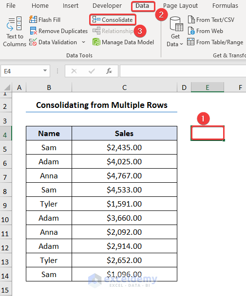
• Initially, select any cell outside the dataset, for example, the E4 cell is chosen below.
• Next, go to Data > Consolidate.

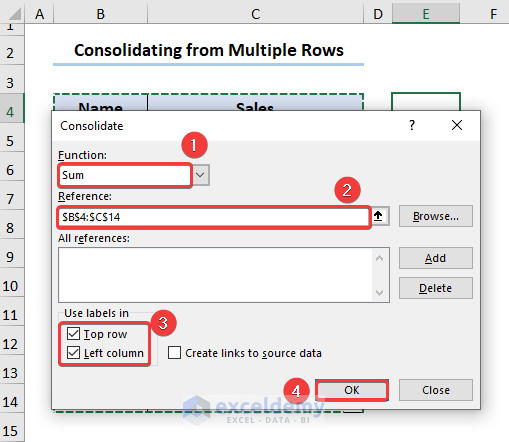
• Now, a dialog box appears where you have to choose the SUM function in the Function
• Following, select the range of cells  $B$4:$C$14 in the Reference
• Then, check the Top row and Left column boxes below.

Finally, the consolidated results appear beside the dataset.

Read More: How to Consolidate Data from Multiple Rows in Excel (4 Quick Methods)

1.2 Consolidation of Multiple Columns 

If you want to consolidate two columns into one then you’ve come to the right place. Allow me to demonstrate.

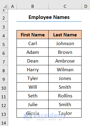
Assuming the following dataset shown in the B4:C14 cells below. Here, the dataset consists of 2 columns with the First Name and the Last Name of the employees.

Steps:

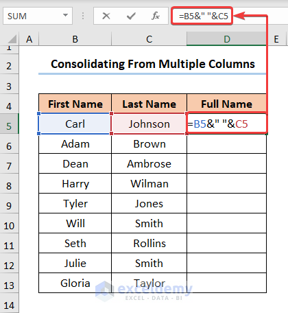
• Firstly, insert a column with the heading Full Name.
• Then, enter the expression in the D5 cell as shown below.

In the above formula, the B5 cell refers to the First Name and the C5 cell indicates the Last Name. Additionally, the Ampersand operator (&) is used to combine the string of text from both the cells.

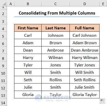
• Next, drag the Fill Handle tool to copy the formula into the cells below.

Lastly, the result is shown in the picture below.

Read More: How to Consolidate Data from Multiple Columns in Excel (7 Easy Ways)

2. Consolidation of Data from Multiple Worksheets

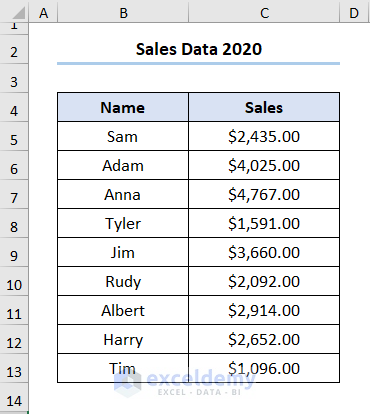
Suppose, we have the Sales Data for 2 years in two separate spreadsheets and we want to merge them into one worksheet. In this case, data consolidation becomes a handy tool. Let’s see it in action.

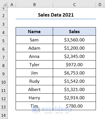
Considering the dataset in the B4:C13 cells. Here, the Employee Names, and their Sales for the year 2020 are shown.

Likewise, the Sales Data for the year 2021 is also provided below.

Steps:

• Firstly, open a new worksheet and select any cell, in this case, the B4 cell is chosen.
• Then, go to Data > Consolidate.

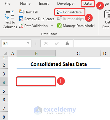
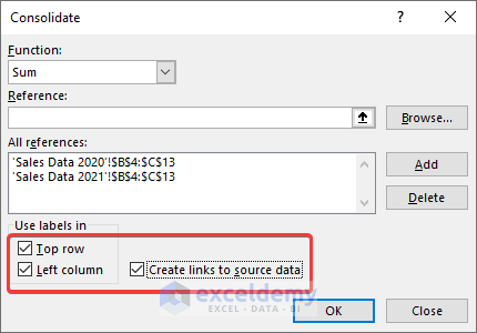
• Now, a dialog box appears, where you have to click on the Reference
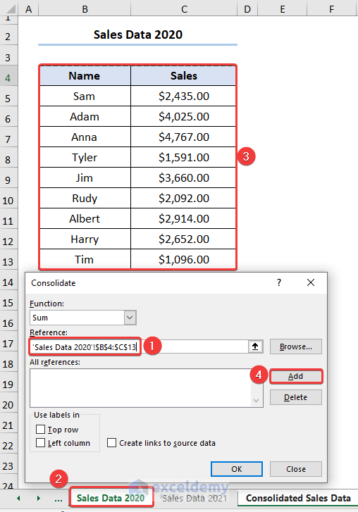
• Next, select the dataset in the B4:C13 range from the Sales Data 2020 worksheet and click Add.

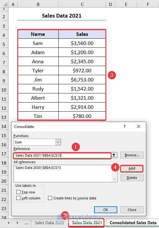
• In a similar fashion, choose the dataset for the Sales Data 2021 spreadsheet and press OK.

Eventually, the outcome should look like the picture shown below.

Admittedly, I have skipped the process of consolidating data from multiple workbooks which you may explore if you wish.

Read More: How to Consolidate Two Sheets into One in Excel (3 Useful Methods)

How to Do Consolidation of Data with Link to Source

Excel allows us to link our consolidated report to the source. Simply put, if we make changes to the source data the report will be updated automatically. Just follow along.

Steps:

• Similar to Case 2, select any cell and go to Data > Consolidate.

• In turn, add the range of datasets from both worksheets.
• Additionally, check the Create links to source data box as shown below.

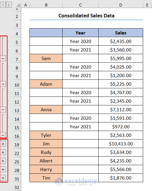
• Just like before, this generates the consolidated report.
• Moreover, the Level Tabs (1 and 2 ) and the Toggle Buttons (+ and – ) appear.

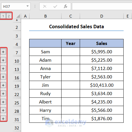
Here, the Level Tabs allow us to drill down into the report while clicking the Toggle Buttons expands the groups.

Conclusion

To conclude, I hope this article helped you understand how to do consolidation in Excel. If you have any queries, please leave a comment below. Also, if you want to read more articles like this, you can visit our website ExcelDemy.