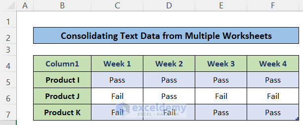
Example 1 – Use the Consolidate Function for Text Data from Multiple Worksheets with the Power Query Tool
- Make sure all worksheets have the same rows and column headers.
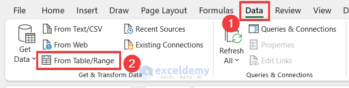
- Go to the Data tab > From Table/Range.
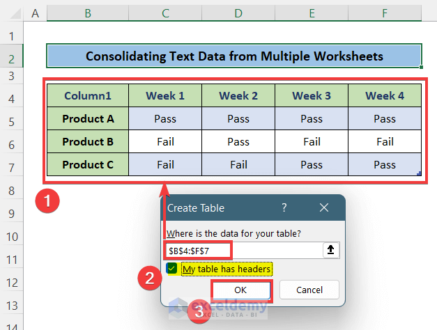
- In “Create Table”, select the data table in the first worksheet.
- Check “My table has headers”.
- Click OK.
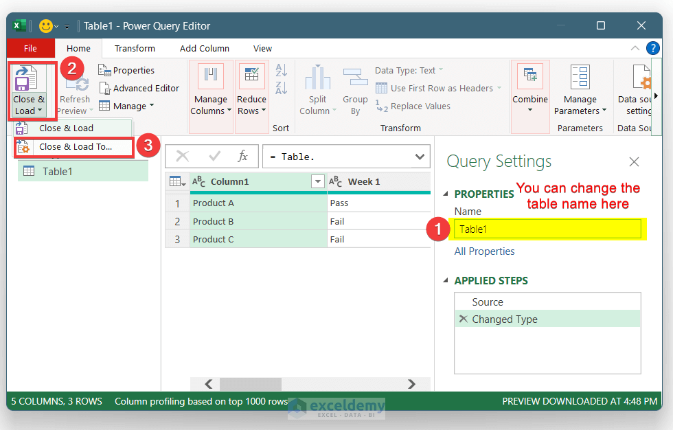
- In the power query window, rename the table.
- Click “Close & Load” and select “Close & Load to”.
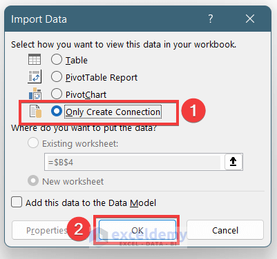
- Select “Only Create Connection” in “Import Data”.
- Click OK.
- Follow the same steps for the remaining worksheet data and create tables in the power query.
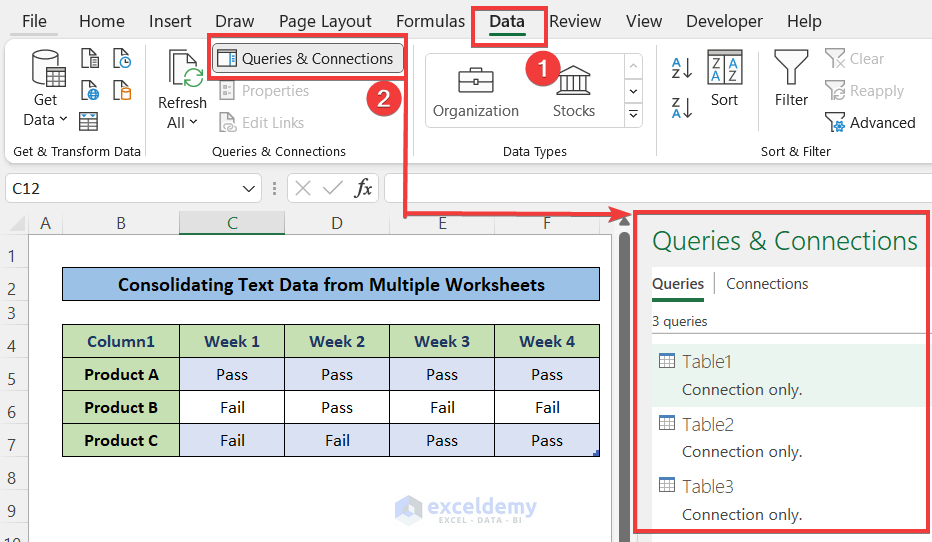
- Go to the Data tab and select Queries & Connections.
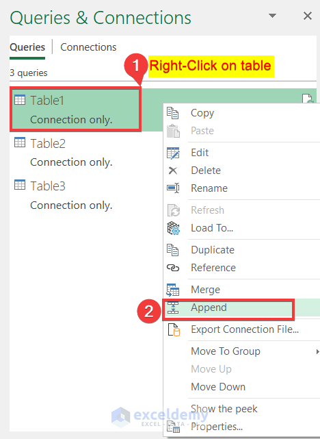
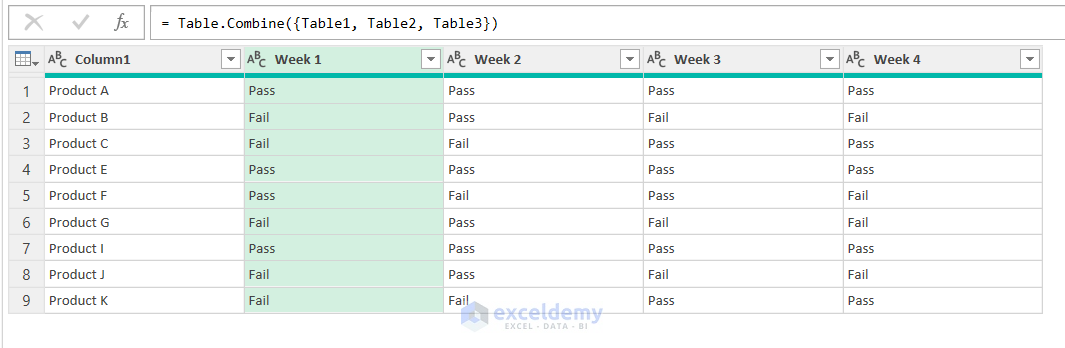
- Right-click Table 1 and select Append.
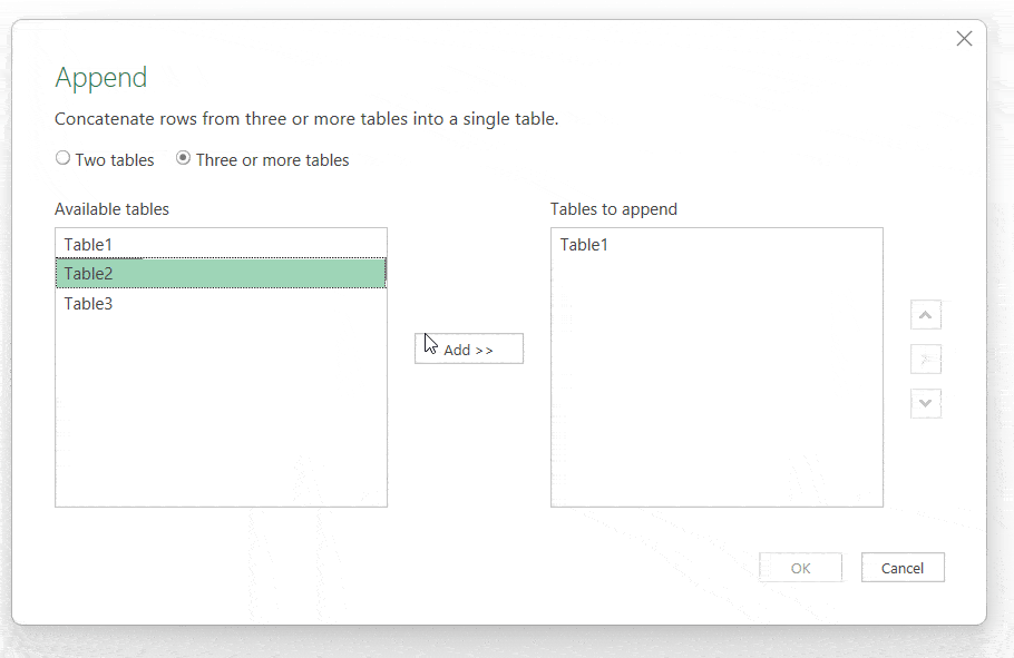
- In the Append window, select three or more tables.
- Add Table 2 and Table 3 in Tables to Append.
- You will see the consolidated text data under the same header.
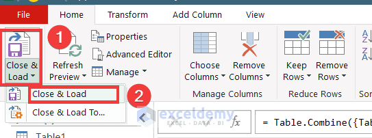
- To import the data to the worksheet, click Close & Load.
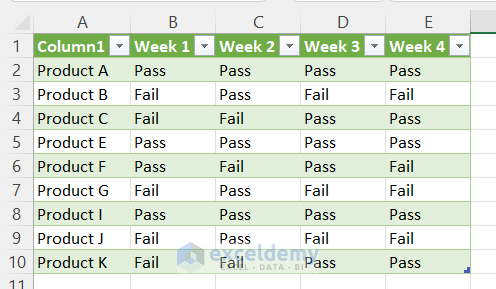
A new worksheet will be created with the consolidated text data.
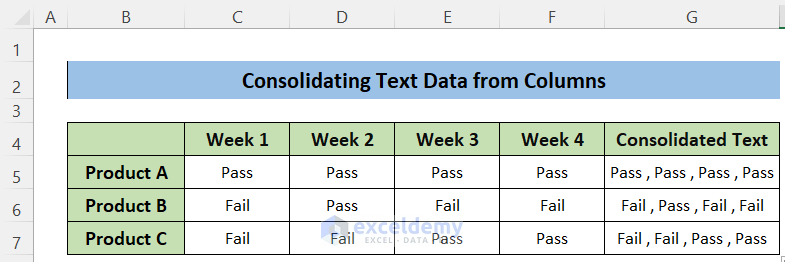
Example 2 – Use the TEXTJOIN Function
- Create a column to get the consolidated text data from the columns.
- Enter the in G5:
=TEXTJOIN( " , ",TRUE,C5:F5)- Drag the Fill Handle icon to copy the formula to the other cells, or use press Ctrl+C and Ctrl+P to copy and paste.
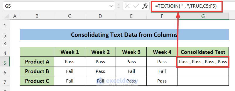
- You will see the consolidated text data with commas as delimiters.
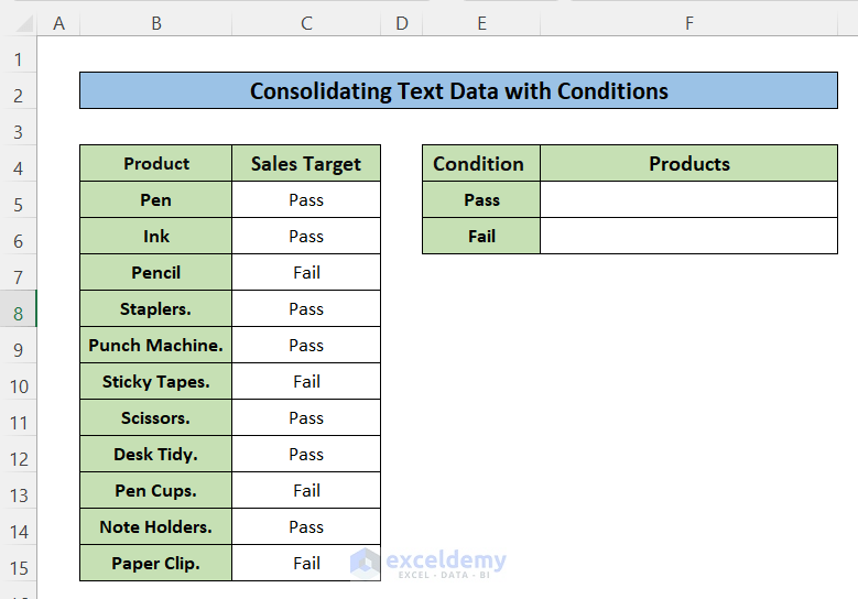
Example 3 – Consolidate Text with a Condition Using the Combination of the TEXTJOIN and FILTER Functions.
- Insert columns to store the consolidated text data for the conditions.
- Set the conditions: Pass and Fail to get the list of products in cells.
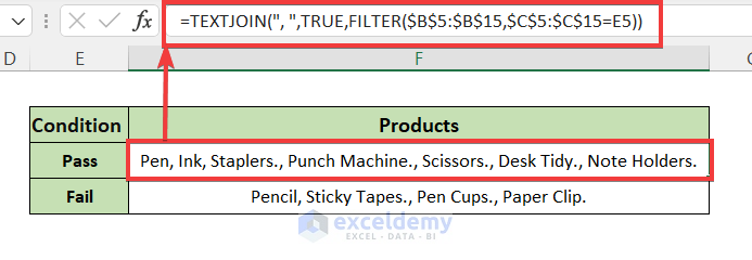
- Enter the formula inl E5.
=TEXTJOIN(", ",TRUE,FILTER($B$5:$B$15,$C$5:$C$15=E5))- It will return the list of products in B5:B15 that meet the filter criteria = “Pass” in C5:C15 with commas as delimiters.
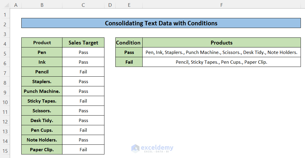
- Drag down the Fill Handle to see the result in the rest of the cells.
Things to Remember
- The Consolidate feature can consolidate number data only.
Download Practice Workbook
Download the practice workbook.
<< Go Back To Consolidation in Excel | Merge Sheets in Excel | Merge in Excel | Learn Excel
Get FREE Advanced Excel Exercises with Solutions!
