How to Create a Linked Consolidation in Excel (2 Useful Methods)

To make a summary report, we often have to consolidate data. But if we don’t create a link between consolidated data and source data then the consolidated data won’t be updated automatically when source data is changed. So it’s an important issue while consolidating data. We can handle this issue in 2 useful ways. In this article, I’ll show those two quick ways to create a linked consolidation in Excel.

Download Practice Workbook

You can download the free Excel workbook from here and practice independently.

2 Ways to Create a Linked Consolidation in Excel

Let’s get introduced to our dataset first. It represents the monthly sales report for three consecutive years in three different regions.

1. Using Formula to Create a Linked Consolidation

First, we’ll apply a formula to create a linked consolidation in excel. We’ll just find the sum of sales using the SUM function for every connected month and region as a summary report. But keep in mind, for this method, the source dataset should be of the same size and same cell reference in every sheet. Otherwise, this method won’t work properly.

Steps:

• In Cell C5, type-

• Then click on the first sales sheet.

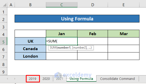
• Next, just select the first sales.

• After that, press and hold the SHIFT key and click the last sales sheet. So it will select all the same cells till the last sheet. No need to select one by one manually.
• Then hit the ENTER button.

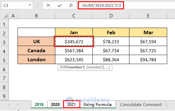
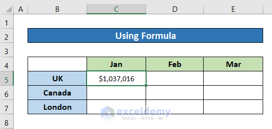
It’s the total sales of January in the UK region for the three consecutive years.

• Later, drag the Fill Handle icon in the right direction to apply the same formula for other months of the UK region.

• Lastly, drag down the Fill Handle icon to apply the formula in the rest two regions.

Then the output will look like the following image.

Now if we change any data, it will be updated automatically. Look, I changed a value in the sales report of 2019- inserted 0 there.

Now go back to the main sheet and see that the output updated automatically.

Read More: How to Automate Consolidation in Excel (with Easy Steps)

2. Using Excel Consolidate Command to Create a Linked Consolidation

There is a dedicated command in Excel named Consolidate to create a linked consolidation. The advantage of it is- there is no need for the same cell references in every sheet, you can place the dataset anywhere.

Steps:

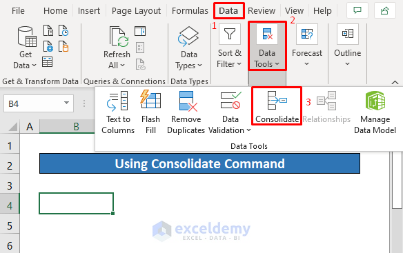
• First, select a cell in a new sheet.
• Then click as follows: Data > Data Tools > Consolidate.

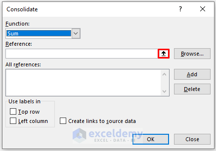
Soon after, a dialog box will open up.

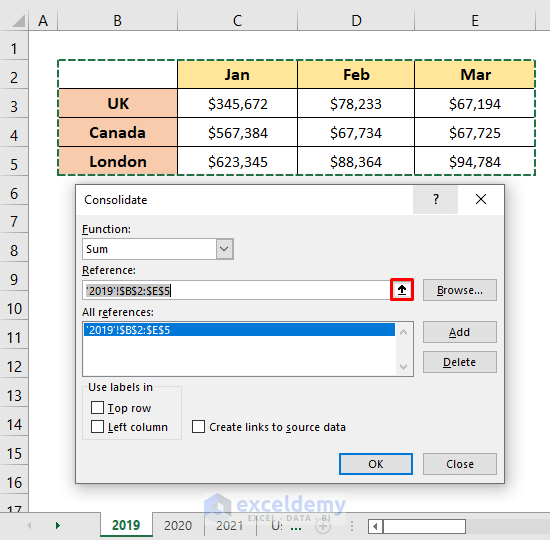
• Select the function from the Function drop-down section that you want to apply. I selected Sum.

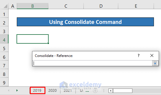
• Later, click on the Open icon from the Reference box.

• Next, go to the first sheet by clicking on it.

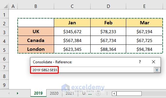
• Then select the data range including the headers by dragging with the mouse
• Press the ENTER button.

• After that, click the Add button.

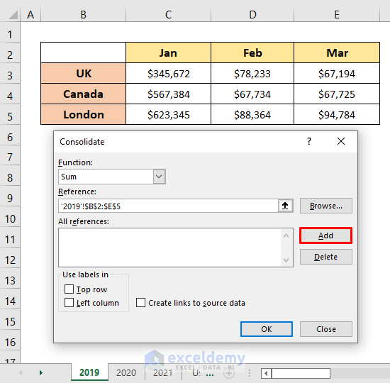
Now see, the reference is added.

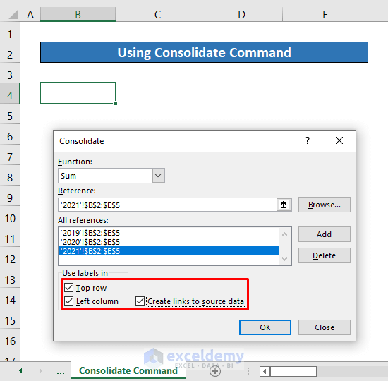
• Again click on the open icon and follow the previous three steps to add the references from the rest of the two sheets.

• Now we have come to the last and most important step. As we have headers along a row and a column, so mark the Top row and Left column option from the ‘Use labels in’ section.
• As we want to create linked consolidation, so mark Create links to source data.
• Finally, just press OK.

Now have a look, we got the same output as the previous method including the Group feature of Excel. But it will not extract formats from the source data. You will have to apply again.

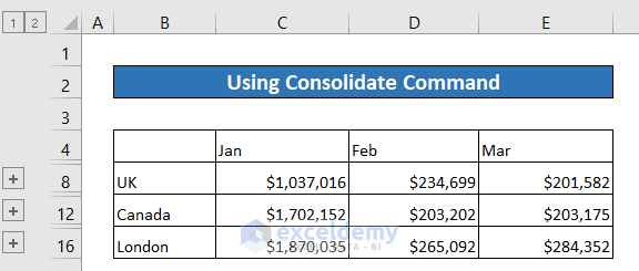
I applied some formats.

• If you click on any plus sign (+) then it will show you the source data of the corresponding region.

See, it’s showing the source data of the UK region. If you press the minus (-) sign then it will be minimized.

• Now let’s check the linking. I inserted zero in Cell C3 of the 2019 sheet.

And yes! The output updated perfectly.

Read More: How to Do Consolidation in Excel (2 Useful Cases)

Conclusion

I hope the above procedures will be good enough to create a linked consolidation in excel. Feel free to ask any questions in the comment section and give me feedback. Visit ExcelDemy to explore more.

Related Articles

• How to Build a Static Consolidation in Excel (2 Suitable Examples)
• Data Validation and Consolidation in Excel (2 Examples)
• How to Consolidate Data from Multiple Columns in Excel (7 Easy Ways)
• Consolidate Function for Text Data in Excel (with 3 Examples)
• How to Remove Consolidation in Excel (2 Handy Methods)
• Consolidate Data in Excel from Multiple Workbooks (2 Methods)
• How to Consolidate Data from Multiple Rows in Excel (4 Quick Methods)