In many cases, you may need to consolidate, merge, or combine data. In Microsoft Excel, you can do such types of tasks in bulk and within seconds. This article demonstrates how to consolidate data in Excel from multiple rows with some quick methods.
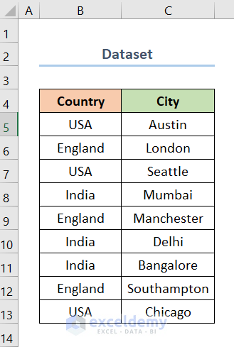
Now, let’s assume you have a dataset with a list of Countries and their Cities. Here, you want to have the multiple rows for Cities consolidated beside their Country. At this point, I will show you two methods using this dataset to do so.
1. Using UNIQUE and TEXTJOIN Functions to Consolidate Data from Multiple Rows in Excel
Using UNIQUE and TEXTJOIN functions is one of the fastest and most convenient ways to consolidate data from multiple rows in Excel. Now, follow the steps below to consolidate data using these functions.
Steps:
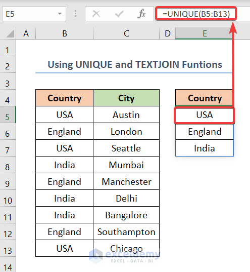
- First, create a new column for Country beside your dataset.
- Next, select cell E5 and insert the following formula.
=UNIQUE(B5:B13)In this case, cell E5 is the first cell of the new column Country. Also, B5 and B13 are the first and last cells of the dataset column Country.
Moreover, we use the UNIQUE function. The syntax of this function is UNIQUE(array, [by_col], [exactly_once]).
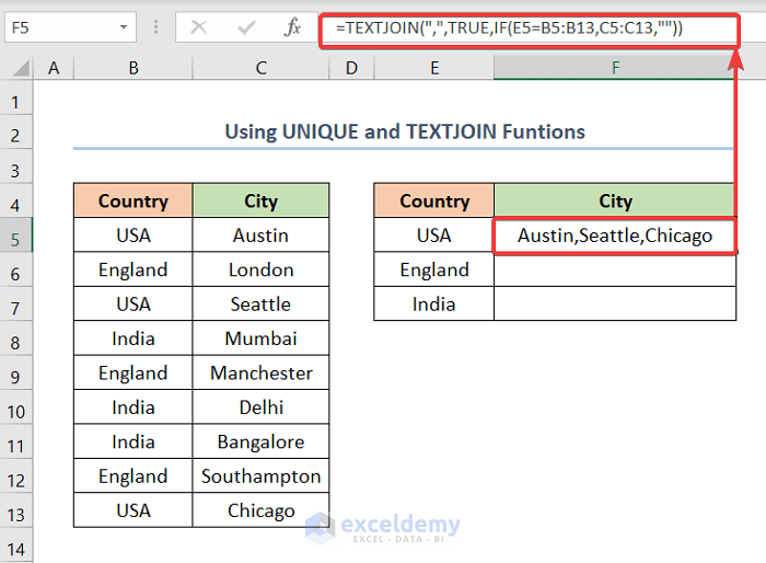
- Then, add another column for consolidated data on the cities.
- After that, click cell F5 and insert the following formula.
=TEXTJOIN(",",TRUE,IF(E5=B5:B13,C5:C13,""))Here, cell F5 is the first cell of the new column City. Also, cells C5 and C13 are the first and last cells of the dataset column City respectively.
Moreover, here, we use the TEXTJOIN function. The syntax of this function is TEXTJOIN(delimiter,ignore_empty,text1,…). Also, we use the IF function.
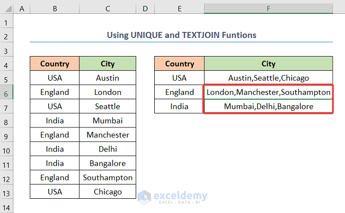
- Finally, drag the Fill Handle for the rest of the column.
2. Using Excel IF Function and Then Sort to Merge Data from Multiple Rows
Another way to consolidate the data from multiple rows in Excel is to use the IF function and the Sort option from the Data tab simultaneously. Now, follow the steps below to do so from the above dataset.
Steps:
- First, select the cell range you want to sort. In this case, it is range B5:B13.
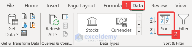
- Then, go to the Data tab > Sort & Filter > Sort A to Z.
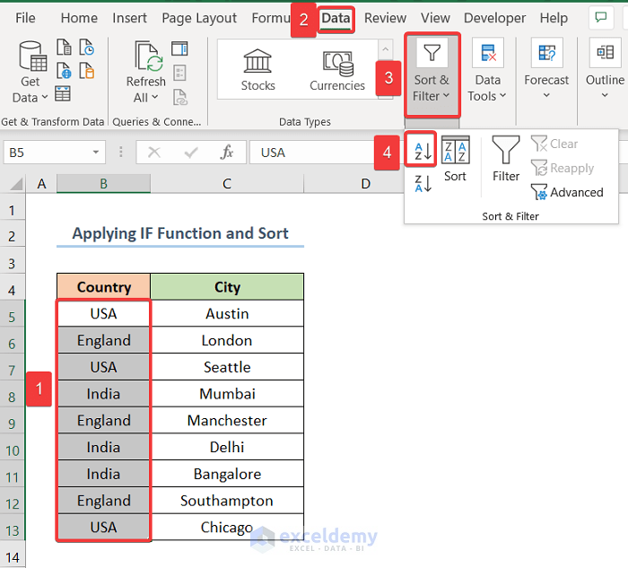
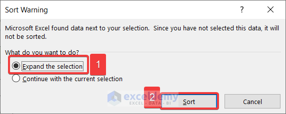
- Now, a Sort Warning box will pop up. At this point, select Expand the selection.
- Next, click on OK.
- Consequently, add another column for Cities.
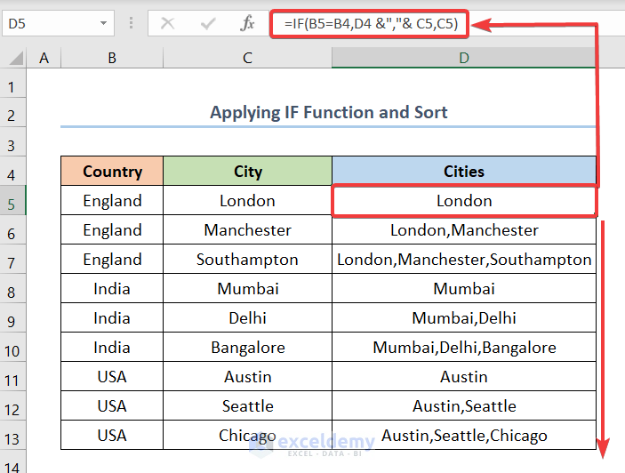
- After that, select cell D5 to insert the following formula, and drag the Fill Handle for the remaining cells of the column.
=IF(B5=B4,D4 &","& C5,C5)In this case, cell D5 is the first cell of the column Cities.
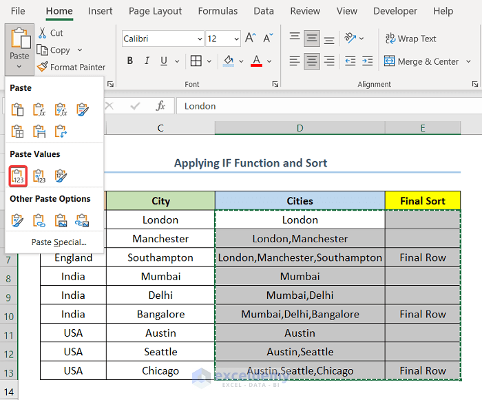
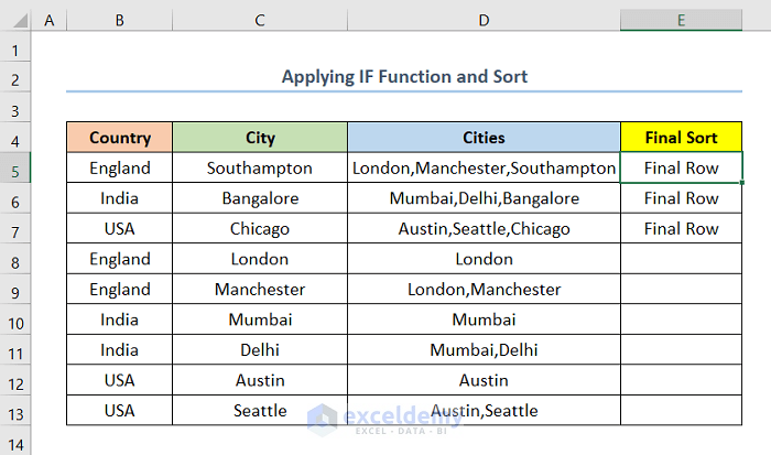
- At this point, insert a new column named Final Sort.
- Then, select cell E5, insert the following formula, and drag the Fill Handle for the remaining column cells.
=IF(B5<>B6,"Final Row","")In this case, B5 and B6 are the first and second cells of the column City respectively. Also, E5 is the first cell of the column Final Row.

- Now, select and copy range D5:E13 and paste them in Values format to remove their formula.
- Next, go to the Data tab > Sort.
- At this point, from Sort by options select Final Sort.
- Then, from the Order options select Z to A.
- Consequently, click OK.

- Now, a Sort Warning box will pop up. At this point, select Expand the selection.
- Next, click on OK.
- At this point, you will have your output as shown in the below screenshot.
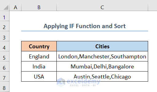
- Finally, delete all extra rows and columns and have your desired output.
3. Consolidate Data from Multiple Rows in Excel with Consolidate Wizard
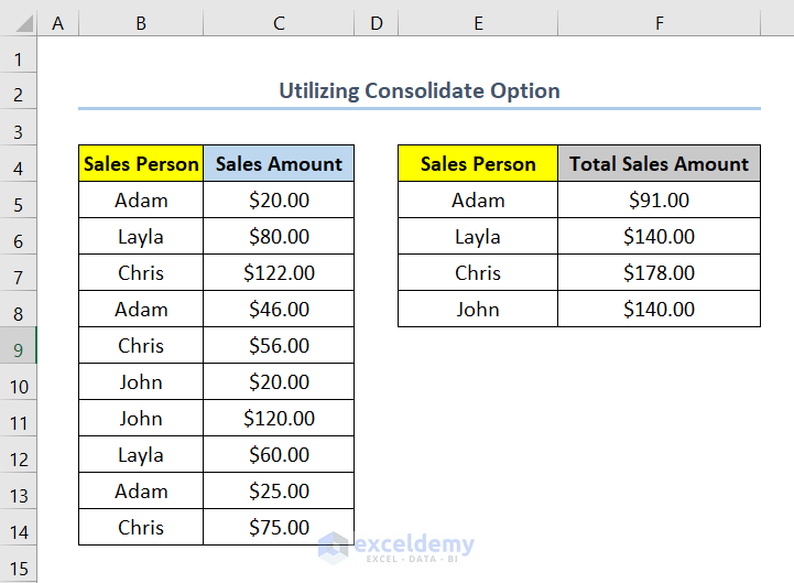
Now, suppose you have a dataset where you have sales made by a few persons on different occasions. At this point, you want to consolidate the data of their sales and get their sum from multiple rows. To do consolidation in Excel, you can follow the steps below.
Steps:
- First, select the cell you want your new data in.
- Second, go to the Data tab.
- Then, select Consolidate from the Data Tools.

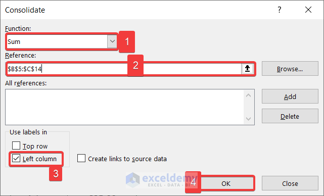
- Then, select Sum from the Function options.
- After that, select the Reference, In this case, it is $B$5:$C$14.
Here, cell B5 is the first cell of the column Sales Person and cell C14 is the last cell of the column Sales Amount.
- Next, pick the Left column from Use labels in.
- Consequently, click on the OK button.
- Finally, you have your consolidated data for sales.
Note: If you want to get your data consolidated based on criteria, first Sort your data according to your criteria and then use the Consolidate option.
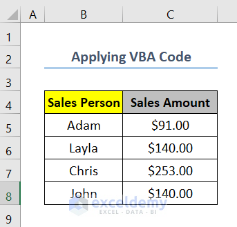
4. Consolidate Data from Multiple Rows with Excel VBA
Also, you can apply VBA code to easily consolidate data from multiple rows in Excel. If you want to do so, you can follow the steps below.
Steps:
- First, press ALT + F11 to open the VBA window.
- Now, select Sheet 7 or the sheet you are working on, and Right-Click on it.
- Next, sequentially select Insert > Module.

- At this point, copy the following code and paste it into the blank space.
'This code will consolidate data from multiple rows
Sub ConsolidateMultiRows()
'Declares Variables
Dim Rng As Range
Dim Dat As Variant
Dim j As Variant
'Creates a InputBox to insert Reference Cell Range
On Error Resume Next
Set Rng = Application.Selection
Set Rng = Application.InputBox("Range", "Enter Your Reference Range", Rng.Address, Type:=8)
'Runs a For loop add all the data for same Sales Person and Updates Screen
Set Dat = CreateObject("Scripting.Dictionary")
j = Rng.Value
For i = 1 To UBound(j, 1)
    Dat(j(i, 1)) = Dat(j(i, 1)) + j(i, 2)
Next
Application.ScreenUpdating = False
'Clears all the extra contents and updates screen
Rng.ClearContents
Rng.Range("A1").Resize(Dat.Count, 1) = Application.WorksheetFunction.Transpose(Dat.keys)
Rng.Range("B1").Resize(Dat.Count, 1) = Application.WorksheetFunction.Transpose(Dat.items)
Application.ScreenUpdating = True
End Sub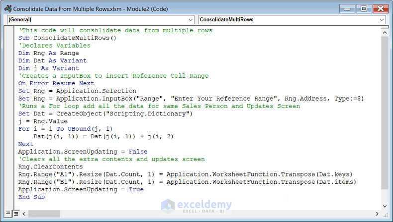
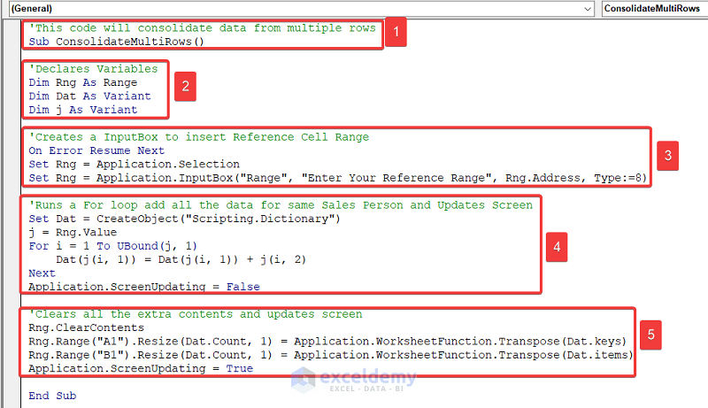
💡 Code Explanation:
In this part, I will explain the VBA code used above. Now, I have divided the code into various sections and numbered them. At this point, I will explain the code section wise.
- Section 1: In this section, we create a new Sub named ConsolidateMultiRows().
- Section 2: Next, we declare different variables.
- Section 3: Here, in this section, we create an InputBox that will ask for our reference range.
- Section 4: We run a For loop for adding the Sales Amount.
- Section 5: Finally, we need to clear all the extra contents and rearrange the cells.
- Now, press F5 and run the code.
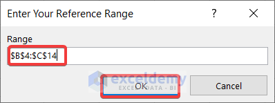
- At this point, a box will appear like the screenshot below.
- Next, insert your reference range
- Finally, click the OK button.
- Lastly, you have your consolidated data like the screenshot below.
Download Practice Workbook
You can download the practice workbook from the link below.
Conclusion
Last but not least, I hope you found what you were looking for in this article. If you have any queries, please drop a comment below.
<< Go Back To Consolidation in Excel | Merge Sheets in Excel | Merge in Excel | Learn Excel
Get FREE Advanced Excel Exercises with Solutions!

Method 1 does not work in Excel 2019. Although lack of the UNIQUE function is easy to overcome, TEXTJOIN does not work as detailed here.
Hi Steven Leblanc
Thanks for your comment. In this article, all the operations are done using Microsoft Office 365 application. That’s why you got a different type of result after using the TEXTJOIN function. If you want to get a similar type of result just like us, you have to update your application from Excel 2019 to Office 365.