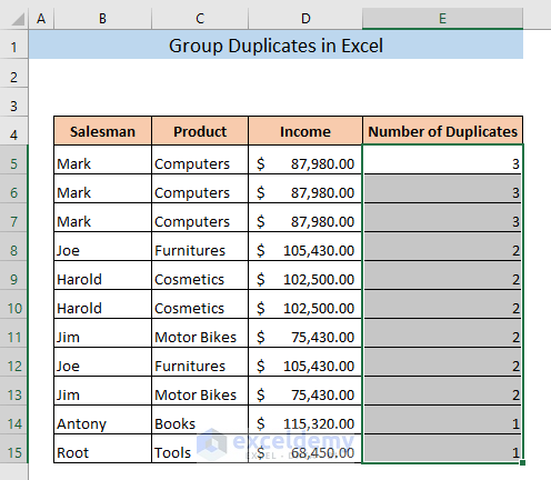
Technique 1 – SUMPRODUCT Function to Group Duplicates
➤ Add the following formula in the first cell of the first empty column next to your dataset (E5),
=SUMPRODUCT(--(B5&C5&D5=$B$5:$B$15&$C$5:$C$15&$D$5:$D$15))The formula will return 1 for each unique data and the number of occurrences for data with duplicate values.
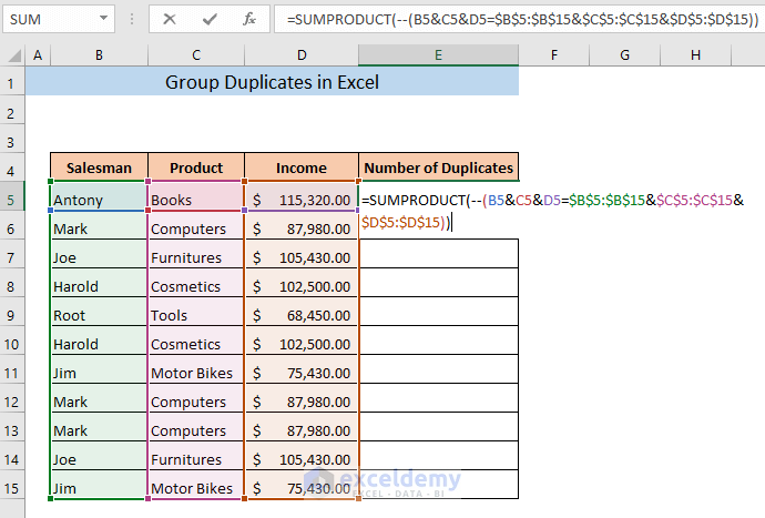
➤ Press ENTER
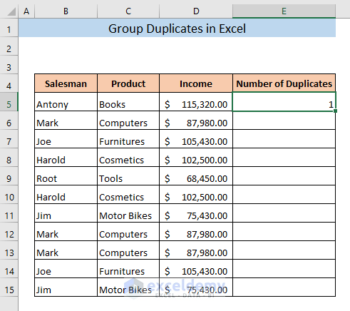
You will get the number of duplicates for the first data. 1 means the data has been found one time in the whole dataset.
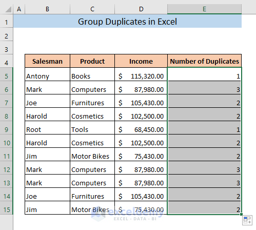
➤ Drag cell E5 to the end of your dataset.
You will get the number of duplicates for all data.
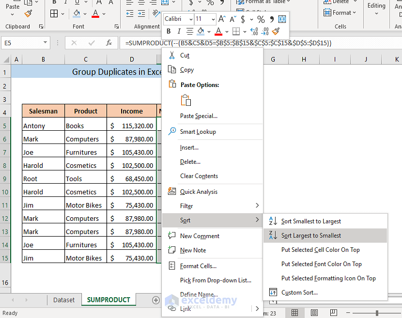
➤ Right click on the selected cells.
A dropdown menu will appear. From this menu,
➤ Click on Sort to Expand it and select Sort Largest to Smallest.
It will rearrange the rows of your dataset and group the duplicates together.
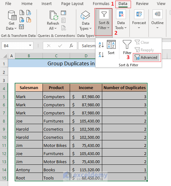
To extract the unique values from this dataset,
➤ Select the entire dataset.
➤ Go to Data > Sort & Filter > Advanced.
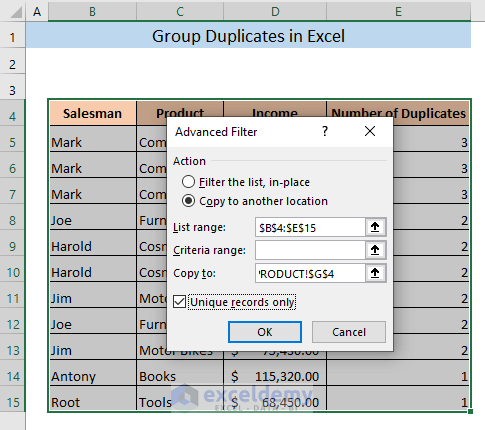
A box named Advanced Filter will appear.
➤ Select the action Copy to another location, select an empty cell in the Copy to box, check the Unique records only box, and click on OK.
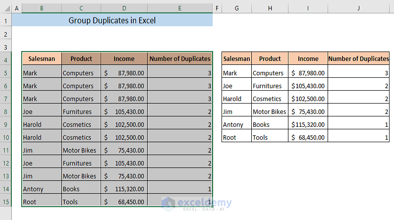
Only the unique values are copied into the new location.
Read More: How to Group Cells with Same Value in Excel
Technique 2 – Group Duplicates with Conditional Formatting
➤ Add the following formula in cell E5,
=B5&C5&D5The formula will combine cells B5, C5, and D5 and will return in cell E5.
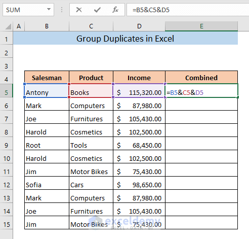
➤ Press ENTER
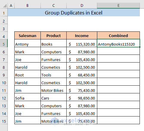
You will get the combination of cells B5, C5, and D5 in cell E5.
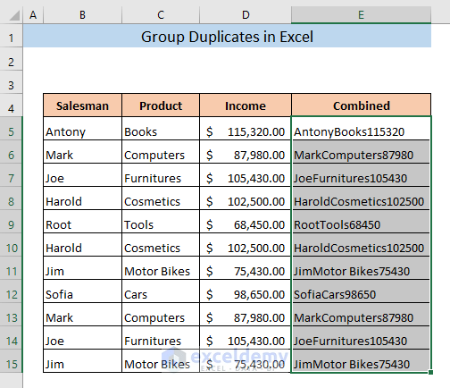
➤ Drag cell E5 to the end of your dataset.
You will get the combined data for all other cells.
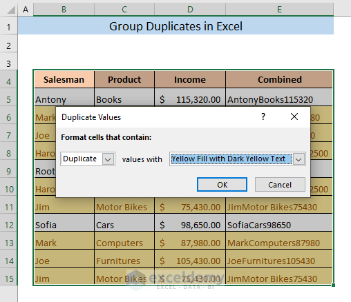
➤ Select your dataset and go to Home > Conditional Formatting > Highlight Cells Rules > Duplicate Values.
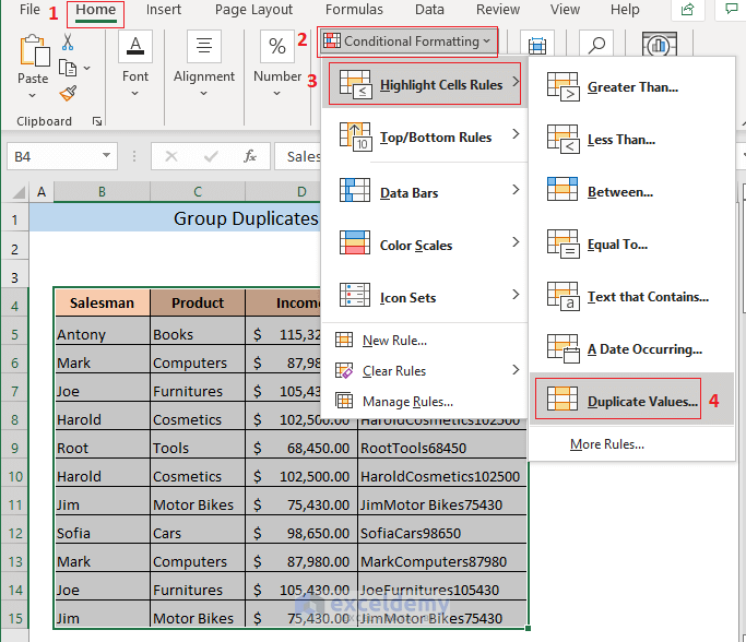
A window named Duplicate Values will be open.
➤ Select a formatting style in the values with box. (For this dataset I’ve chosen Yellow Fill with Dark Yellow Text).
➤ Press OK.
➤ Go to Home > Editing > Sort & Filter > Filter.
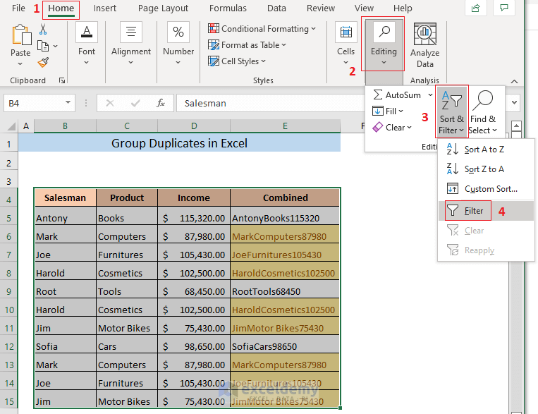
Filter arrows will appear next to each column header.
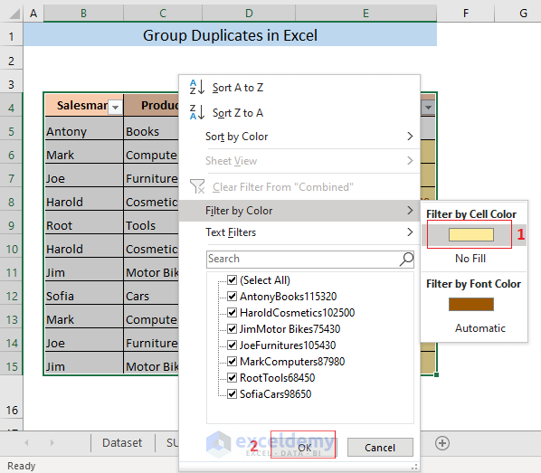
➤ Click on the arrow next to Combined.
A filtering menu will appear,
➤ Go to Filter by Color and select the formatting cell color (Yellow) from Filter by Cell Color. Click on OK.
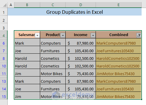
All the duplicates in your dataset will be grouped together.
Read More: How to Group Similar Items in Excel
Technique 3 – Group Duplicates by Combining COUNTIFS and IF Functions
➤ Add the following formula in cell E5,
=IF(COUNTIFS($B$5:$B$15,B5,$C$5:$C$15,C5,$D$5:$D$15,D5)=1,"Unique","Duplicates")The formula will return Unique if the data of row 5 has no other copy and Duplicates if the data of row 5 matches with the data of any other rows.
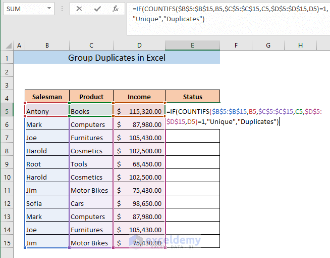
➤ Press ENTER.
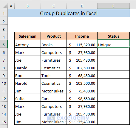
Cell E5 will show Unique, which means the data of row 5 is unique.
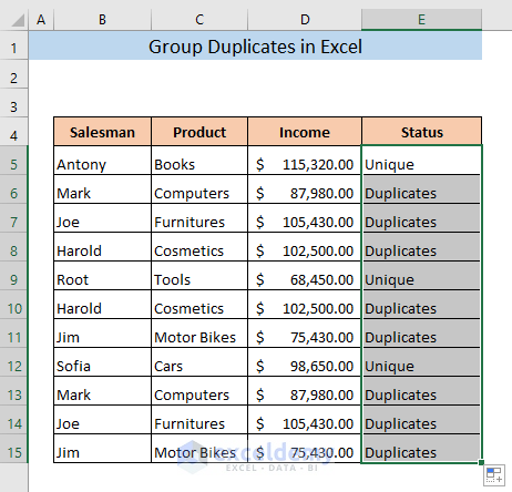
➤ Drag cell E5 to the end of your dataset.
➤ Go to Home > Editing > Sort & Filter > Filter.
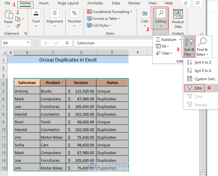
Filter arrows will appear next to the column headers.
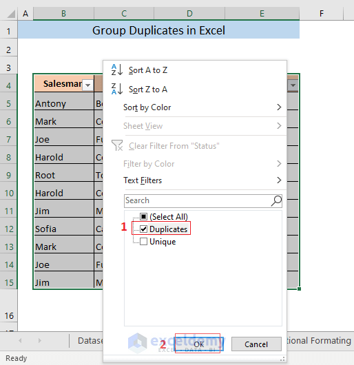
➤ Click on the downward arrow of the column header Status.
A filtering menu will appear.
➤ Check on Duplicates and click on OK.
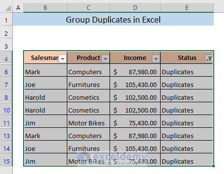
All the duplicates will get grouped together.
To get the same values grouped together,
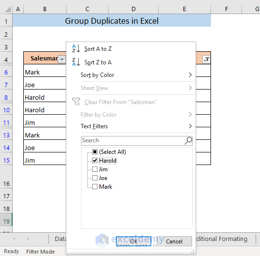
➤ Click on the arrow next to Salesman column (You can also produce the same result by selecting any other columns except the Status column)
It will open the filtering menu.
➤ Check a single name from the list and click on OK.
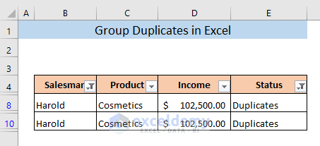
The same values will be grouped together.
Download Practice Workbook
Related Articles
- How to Group Time Intervals in Excel
- How to Remove Grouping in Excel
- How to Group and Ungroup Columns or Rows in Excel
- How to Use Grouping and Consolidation Tools in Excel
- How to Create Multiple Groups in Excel
<< Go Back to Group Cells in Excel | Outline in Excel | Learn Excel
Get FREE Advanced Excel Exercises with Solutions!
