How to Collapse Columns in Excel (6 Easy Ways)

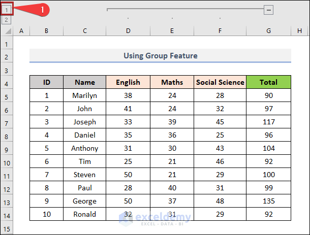
The collapse columns feature in Excel hides the marked columns from being displayed. We will use the sample dataset below to collapse columns D, E, and F.

Method 1 – Using Group Feature to Collapse Columns in Excel

Steps

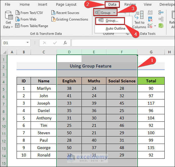
• Select the columns you want to collapse.
• Go to the Data tab.
• Select the Group drop-down on the Outline group.
• Select Group from the drop-down list.

• The above steps will make the selected columns grouped as indicated on the upper side as shown in the image below.

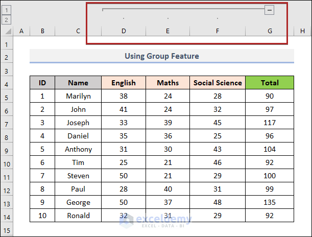
• Click on the negative (-) sign.

• Columns D:F will be collapsed.

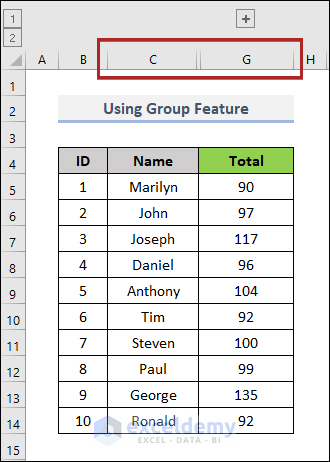
• Click on the plus (+) sign at the top of Column G.

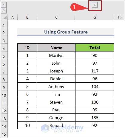
• You can expand or collapse columns using the plus (+) or negative (–) sign.
• Click on button 1 on the top left side as shown in the image below.

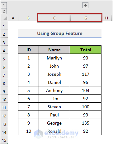
• The three columns in our dataset have collapsed.
• You will notice that Column C and Column G are located side by side.

Method 2 – Applying Context Menu to Collapse Columns in Excel

Steps

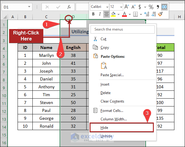
• Select columns in the D:F
• Right-click anywhere on the selected range.
• Select the Hide option from the context menu.

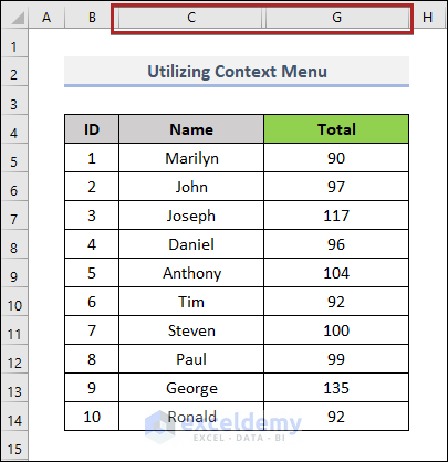
• It will collapse columns D, E, and F.

Method 3 – Collapse Columns with Excel Ribbon

Steps

• Select columns in the D:F range.
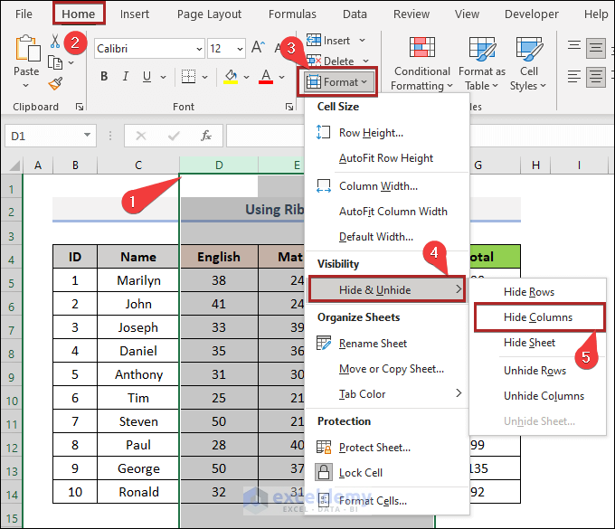
• Go to the Home tab.
• Select the Format drop-down on the Cells group.
• Click on the Hide & Unhide batch under the Visibility section.
• Select Hide Columns from the available options.

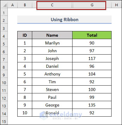
• Columns D:F will be hidden.

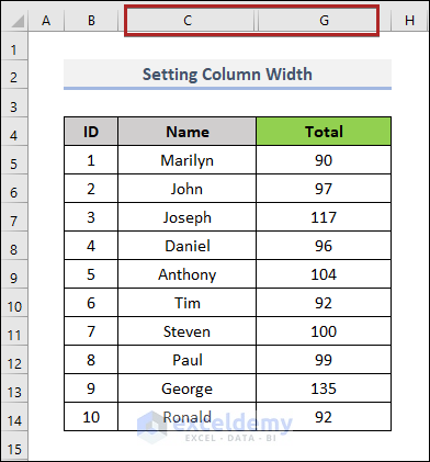
Method 4 – Setting Column Width to Collapse Columns in Excel

Steps

• Select the columns D:F that need to be collapsed.
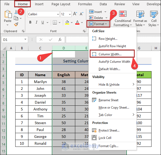
• Move to the Home tab.
• Select the Format drop-down on the Cells group.
• Click Column Width from the options.

• Enter 0 in the Column Width box.
• Click OK.

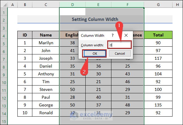
• Columns D:F will be collapsed.

Read More: How to Hide Columns in Excel with Minus or Plus Sign

Method 5 – Applying Keyboard Shortcut to Collapse Columns

Steps

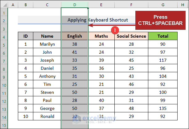
• Click on any cell of Column D.
• Press the CTRL+SPACEBAR.
• This will select the whole column.

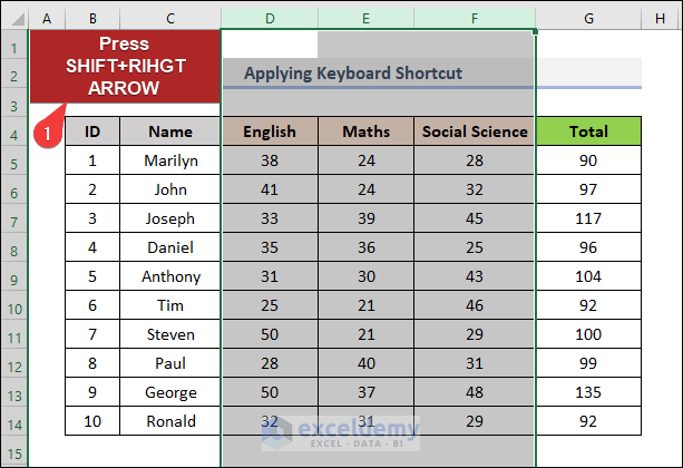
• Press the SHIFT key and tap the RIGHT ARROW (→) key twice to select from Column D to Column F.

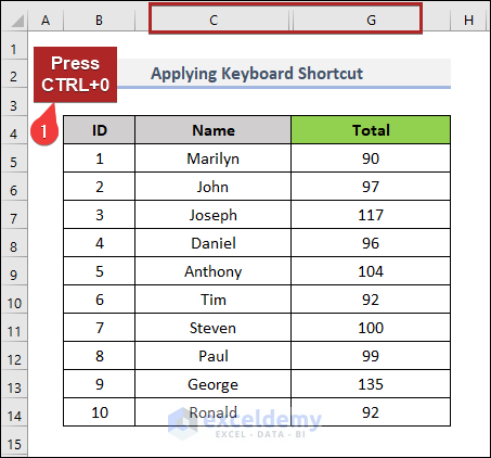
• Press CTRL+0 on your keyboard to get the desired result.

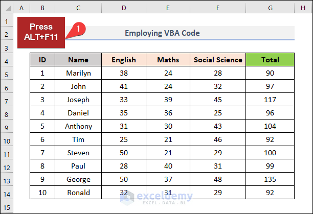
Method 6 – Applying VBA Code to Collapse Columns in Excel

Steps

• Press ALT+F11.

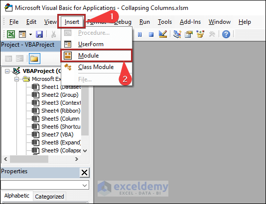
• Go to the Insert tab in the Microsoft Visual Basic for Applications window.
• Select Module from the options.

• Enter the following code in the Module.

Sub Collapse_Columns()
    Range("D:F").EntireColumn.Hidden = True
End Sub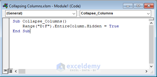

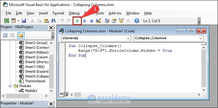
• Click on Run or press the F5 key on your keyboard.

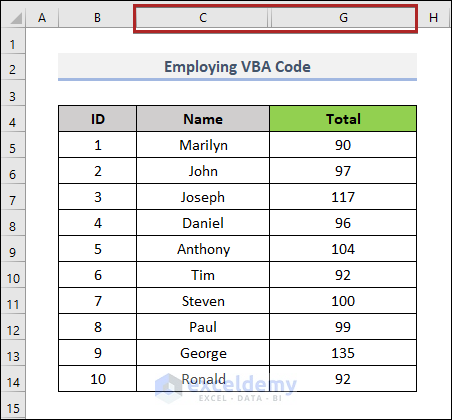
• Return the worksheet.
• The worksheet will look like the one below.

How to Expand Collapsed Columns in Excel?

Steps

• Select Column C and Column G.
• Go to the Home tab.
• Select the Format drop-down on the Cells group.
• Click on the Hide & Unhide batch under the Visibility section.
• Select Unhide Columns from the options.

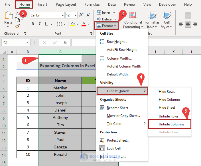
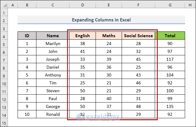
• The previously collapsed columns D:F will be expanded.

How to Collapse Rows in Excel?

Step 1: Prepare a Suitable and Structured Dataset

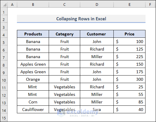
We’ll collapse the rows which contains the orders of Fruit in the sample dataset below.

Step 2: Use Group Feature

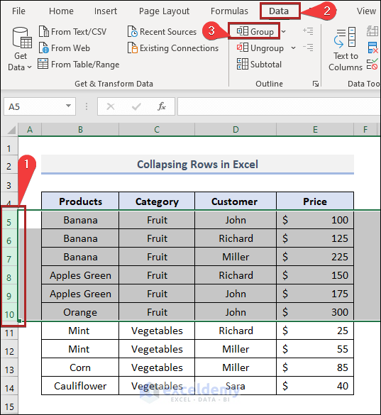
• Select the rows containing orders for the Category- Fruit (rows 5:10).
• Go to the Data tab.
• Select the Group option on the Outline group.

Step 3: Switch Between (+) and (-) Sign

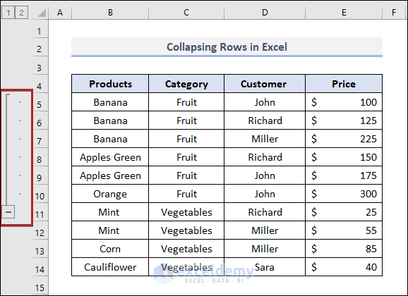
• The above steps will make the selected rows grouped as indicated on the left side as shown in the image below.

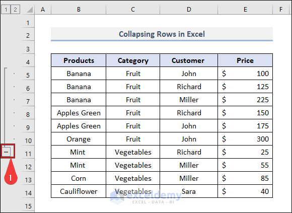
• Click on the minus (-) sign shown in the image below.

• Rows 5:10 will be collapsed.

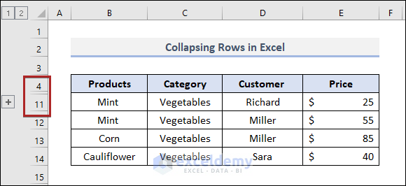
• You can expand these rows by following the steps shown above.

Download Practice Workbook

Related Articles

• How to Group and Hide Columns in Excel
• Excel Hide Columns Based on Cell Value without Macro

<< Go Back to Hide Columns | Learn Excel