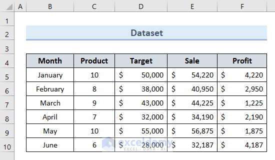
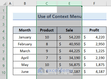
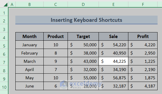
Dataset Overview
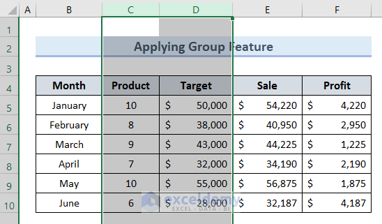
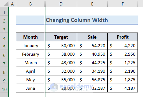
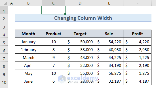
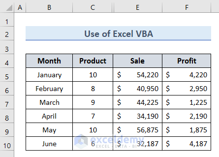
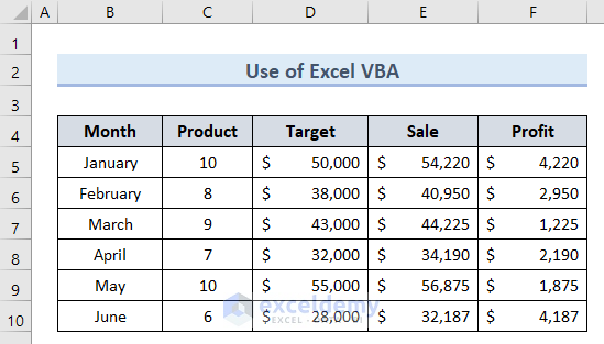
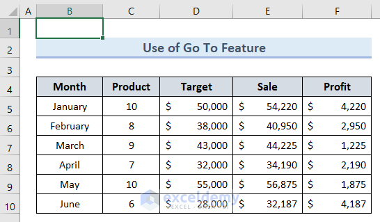
To demonstrate these methods, we’ve prepared a dataset showing information about targets, sales, and profits for a set of products during the first half of the year in a company.
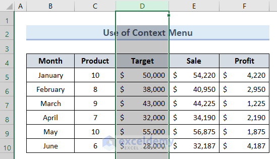
Method 1 – Use Context Menu to Hide and Unhide Columns
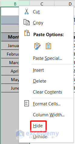
- Select the column you want to hide (e.g., Column D).
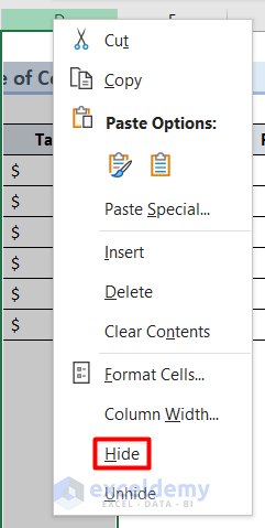
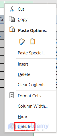
- Right-click on the selected column and choose Hide from the Context Menu.
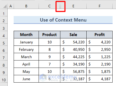
- Column D will no longer be visible in the worksheet.
- You’ll notice a double line on the headings bar, indicating a hidden column.
- To unhide column D, select adjacent columns C and E.
- Right-click and choose Unhide from the Context Menu.
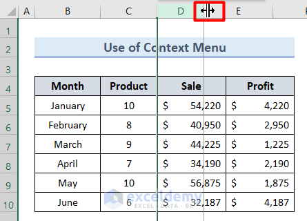
- Alternatively, drag the cursor icon to the right to reveal the hidden column.
Read More: How to Hide Columns with Button in Excel
Method 2 – Hide and Unhide Columns with Format Tool
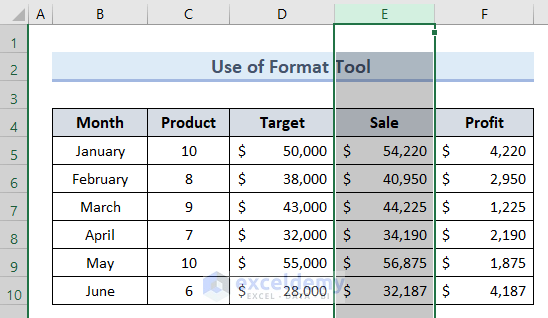
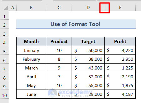
- Select the column you want to hide (e.g., Column E).
- If hiding multiple columns, press Ctrl and select the desired columns.
- Go to the Home tab and click Format under the Cells group.
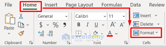
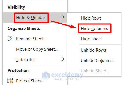
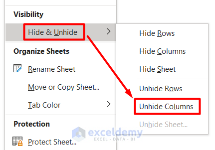
- Choose Hide & Unhide from the Visibility section of the Format drop-down.
- Select Hide Columns.
- Column E will be hidden, indicated by double lines in the headings bar.
- To unhide, select adjacent columns C and E.
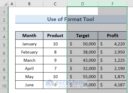
- Go to the Format drop-down and choose Unhide Columns.
Read More: Hide Columns with No Data in Excel
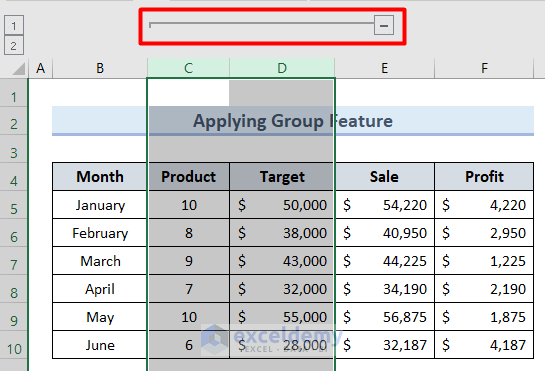
Method 3 – Apply Group Feature to Hide and Unhide Columns
- Select columns C and D.
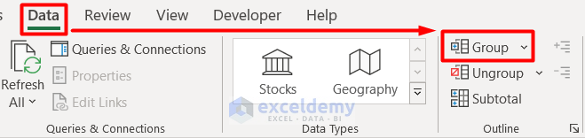
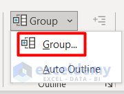
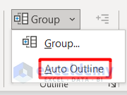
- Go to the Data tab and choose Group under the Outline section.
- The Group feature activates, grouping columns C and D.
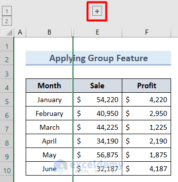
- Click the Minus (–) icon to hide the columns.
- To unhide, click the Plus (+) icon.
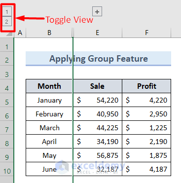
- You can also use the toggle view (click 1 to hide and 2 to unhide).
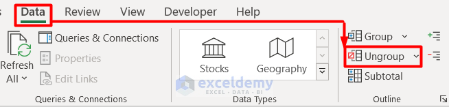
- To disable this feature, go to the Home tab and select Ungroup under the Outline section.
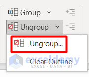
Note: You can also use the Auto Outline tool in the Group feature if your dataset has the SUM function or the SUBTOTAL function.
Method 4 – Insert Keyboard Shortcuts
- Select any cell or adjacent cells (e.g., cell E7).
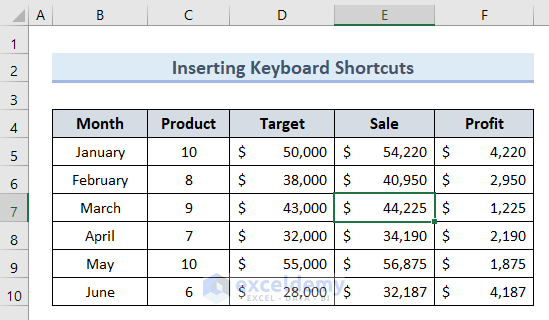
- Press Ctrl + 0 to hide Column E.
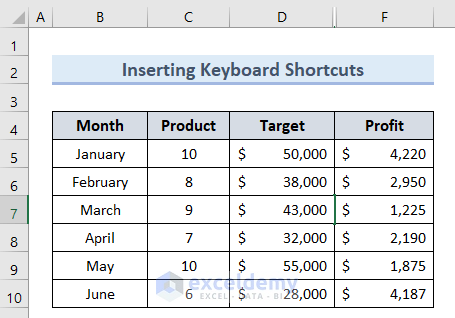
- To unhide, press Alt and type H + O + U + L sequentially on your keyboard.
- It will unhide column E as shown in the image below:
Read More: How to Hide Columns Without Right Click in Excel
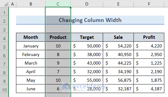
Method 5 – Change Column Width to Hide and Unhide Columns
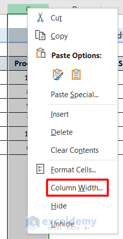
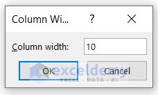
- Select column C or more than two columns if desired.
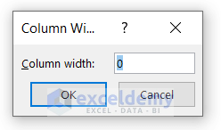
- Right-click and choose Column Width.
- In the new window, type 0 as the column width and press OK.
- The column is now hidden.
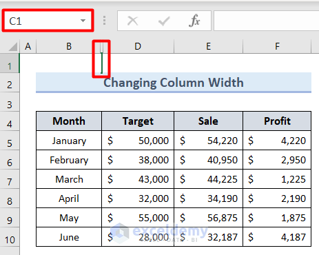
- To unhide it, select any cell and type the cell reference of the hidden column in the Name box (e.g., C1).
- You’ll see a cursor icon over the hidden column.
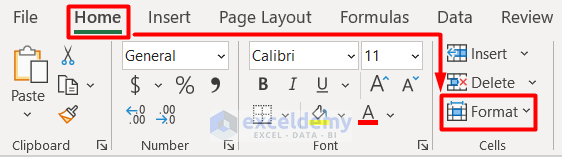
- Go to the Home tab, click Format under the Cells group, and select Column Width from the drop-down.
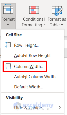
- Type a numeric value to determine the hidden column width and press OK.
- Column C will be unhidden.
Read More: How to Hide Multiple Columns in Excel
Method 6 – Hide and Unhide Columns with Excel VBA
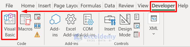
- Go to the Developer tab and select Visual Basic under the Codes group.
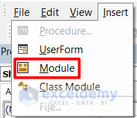
- In the Visual Basic window, choose Module from the Insert section.
- Insert the following code on the blank page:
Sub HideColumns()

    Columns("D").EntireColumn.Hidden = True

End Sub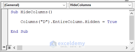
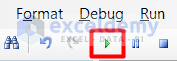
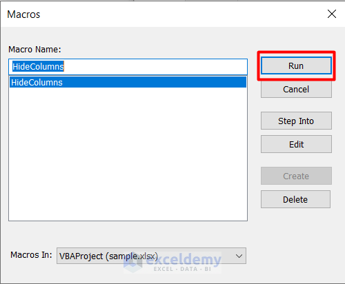
- Click the Run Sub button or press F5 on your keyboard.
- Column D will be hidden.
- To unhide it, create a new Visual Basic page and insert this code:
Sub UnhideColumns()

    Cells.EntireColumn.Hidden = False

End Sub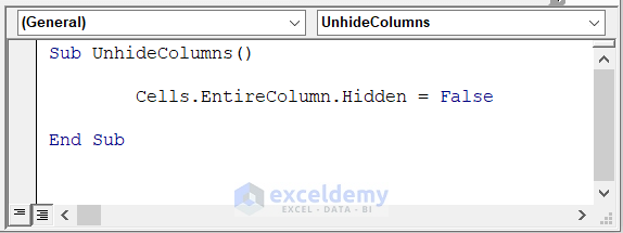
- Run this code with a similar procedure to unhide column D.
Note: To hide more than one column, use this code. Here the column range is variable according to the dataset. For example, we have taken column range A:C.
Sub HideMultipleColumns()

    Columns("A:C").EntireColumn.Hidden = True

End Sub
Method 7 – Use Go To Feature to Hide and Unhide Columns
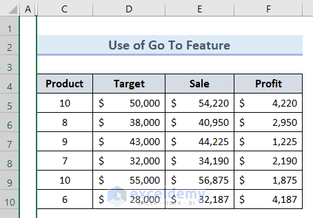
- Select column B and right-click on it.
- Click Hide to hide column B.
- You can see that column B is hidden.
- To unhide it, go to the Home tab and click Find & Select.
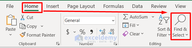
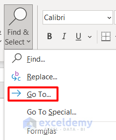
- Choose Go To from the drop-down.
- Insert the reference as B1 in the Go To window (since our hidden column is B) and press OK.
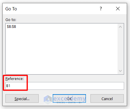
Note: In the case of more than one column, type Reference as a range of columns. For example, type B:C as the reference.
- If the hidden column is still not visible:
- Go to the Home tab, select Format under the Cells group, and click Unhide Columns.


- You will be able to see the hidden column B.
Read More: How to Hide Extra Columns in Excel
How to Check the Number of Hidden Columns in Excel?
- Go to the File tab on the Excel ribbon.
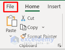
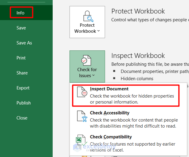
- Navigate to Info and click Check for Issues.
- Select Inspect Document from the drop-down.
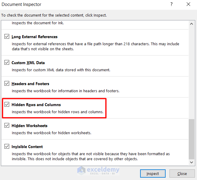
- Choose your preferred option regarding saving the file.

- In the Document Inspector window, ensure that Hidden Rows and Columns are marked.
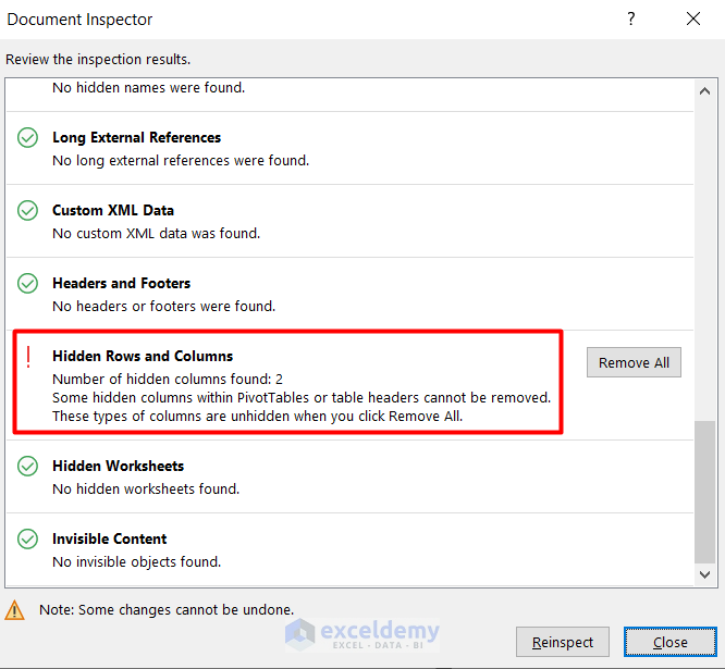
- Click Inspect to find the result of hidden columns in the worksheet.
- You will find the result of hidden columns in this worksheet.
Download Workbook
You can download the practice workbook from here:
Related Articles
- How to Unhide Columns in Excel All at Once
- Unhide Columns Is Not Working in Excel
- Unhide Columns in Excel Shortcut Not Working
<< Go Back to Hide Columns | Learn Excel
Get FREE Advanced Excel Exercises with Solutions!
