Method 1 – Using Excel Ribbon to Group and Hide Columns in Excel
Steps:
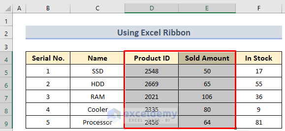
- To hide the Product ID and Sold Amount, you need to group them first.
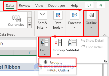
- Go to the Data tab in the Ribbon and select Group in the Outline section.
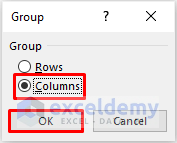
- A selection window will appear. Select Columns and click OK.
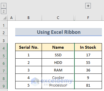
- A “-” mark appears on top of the sheet. This indicates our grouping is done.
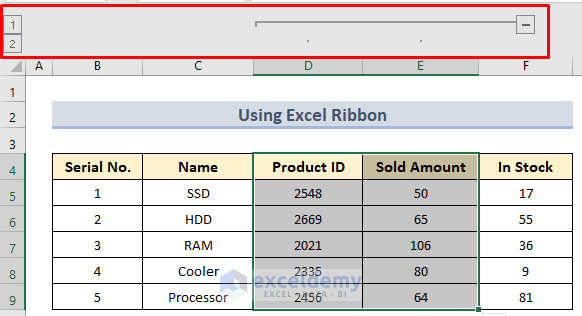
- Click the “-” sign to hide the columns. The “+” sign indicates the grouped columns are hidden and we can expand.
Method 2 – Use of Excel Keyboard Shortcuts to Group and Hide Columns
Steps:
- Select the columns. In our case, we will select columns D and E.
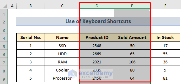
- Press Shift+Alt+Right Arrow.
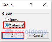
- The Group box opens, select Columns and press OK.
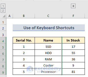
- The columns are grouped. Click on the dash (-) button to hide it.
Method 3 – Applying VBA to Group and Hide Columns in Excel
Steps:
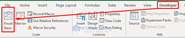
- Choose which columns to group and hide. We will group and hide columns E and F. Go to the Developer tab in the Ribbon and choose Visual Basic. A window will appear. Or open it by pressing Alt+F11.
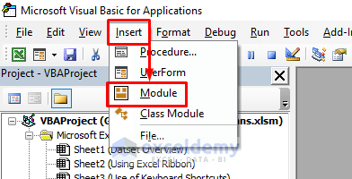
- Select Insert and choose Module. A window will open.
- Enter the following code:
Sub G_H()
Columns("E:F").Group
End Sub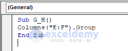
You can give the respective field sequence you need instead of E and F.
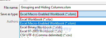
- Press Ctrl+S to save the file as an Excel Macro-Enabled Workbook or as a .xlsm
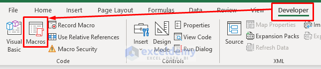
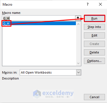
- Go to the Developer tab and select Macros. A window named Macro will appear.
- Select G_H and click Run.
- The columns are grouped. Hide it by pressing the “-”.
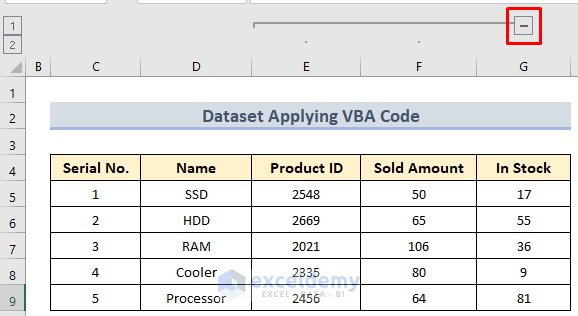
- Pressing the “–” sign will give us the following result.

Read More: How to Hide Columns in Excel with Minus or Plus Sign
How to Hide Columns in Excel Without Grouping?
Method 1 – Using Excel Context Menu to Hide Columns Without Grouping
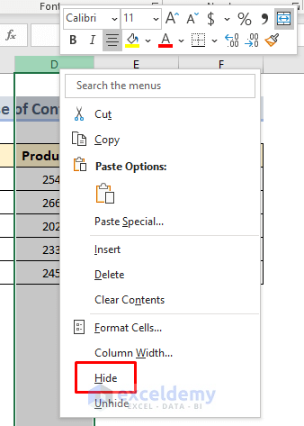
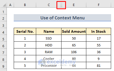
In this method, we select a column that we will hide. Right-click to get the Context menu. Select Hide and the column will be hidden.
Identify the hidden column with the sign in between two columns as shown below.
Method 2 – Use of Keyboard Shortcut to Hide Columns in Excel Without Grouping
Select a column and press Ctrl+O.
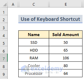
We hid the B, D, and F columns.
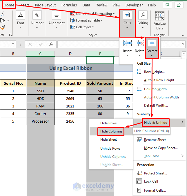
Method 3 – Using Excel Ribbon to Hide Columns
Select a column or multiple columns go to Home tab, click on Cells and choose Format. In format select Hide & Unhide. We will select Hide Columns.
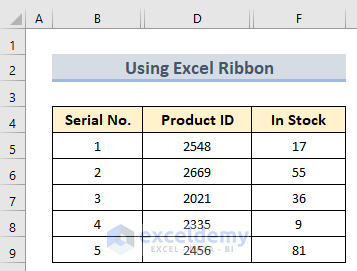
The selected columns will be hidden.
Download Practice Workbook
Related Articles
<< Go Back to Hide Columns | Learn Excel
Get FREE Advanced Excel Exercises with Solutions!
