Hide Columns with No Data in Excel – 4 Methods

This is the sample dataset.

To hide all columns except for the first 3:

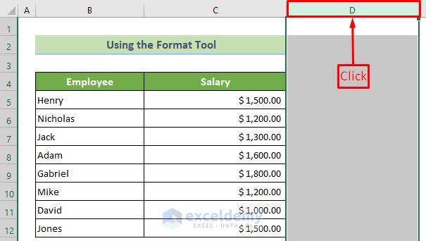
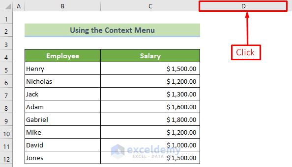
Method 1 – Hide Columns with No Data Using the Format Tool

Steps:

• Click the header of column D.

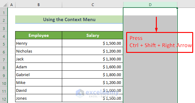
• Press Ctrl + Shift + Right arrow.

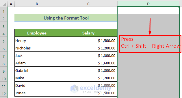
You selected all unused columns.

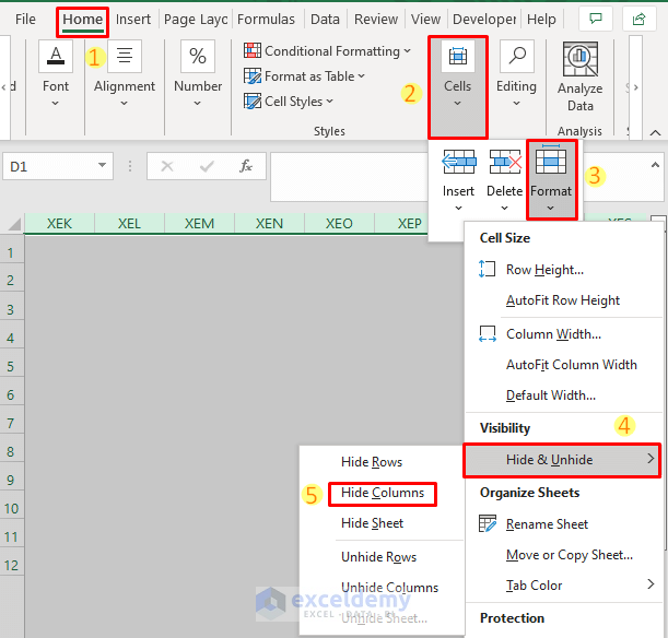
• Go to the Home tab >> Cells >> Format >> Hide & Unhide >> Hide Columns.

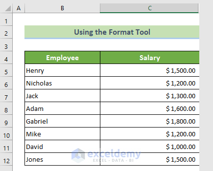
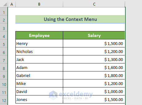
This is the output.

Read More: How to Hide Columns with Button in Excel

Method 2 – Hide Columns with No Data Using the Hide Command

Steps:

• Click the header of column D.

• Press Ctrl + Shift + Right arrow.

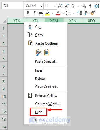
• Place the cursor on any column header.
• Right-click.
• Choose Hide.

This is the output.

Read More: How to Hide Multiple Columns in Excel

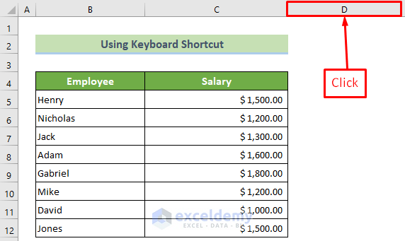
Method 3 – Use a Keyboard Shortcut to Hide Columns with No Data

Steps:

• Click the header of column D.

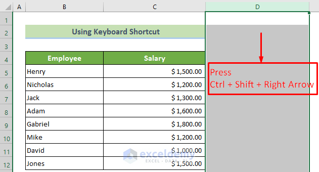
• Press Ctrl + Shift + Right Arrow.

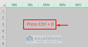
• Press Ctrl + 0.

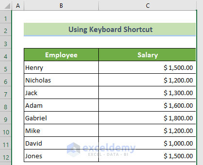
This is the output.

Read More: How to Hide Columns Without Right Click in Excel

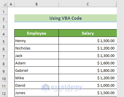
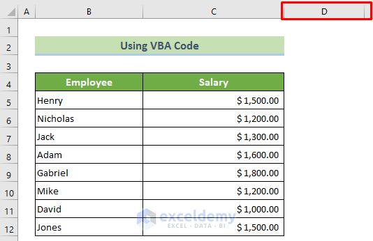
Method 4 – Apply a VBA Code

Steps:

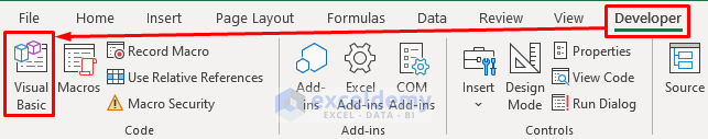
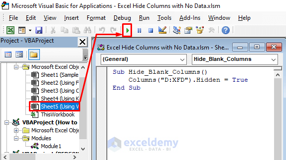
• Go to the Developer tab >> Visual Basic.

• In the Microsoft Visual Basic for Applications window, click Sheet5 in Microsoft Excel Object.
• Enter the following code in the code window.

Sub Hide_Blank_Columns()
    Columns("D:XFD").Hidden = True
End Sub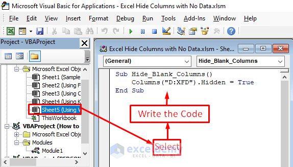

• Press Ctrl + S to save the code.
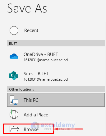
• Go to the File tab.

• Choose Save As in the File tab.

• Click Browse.

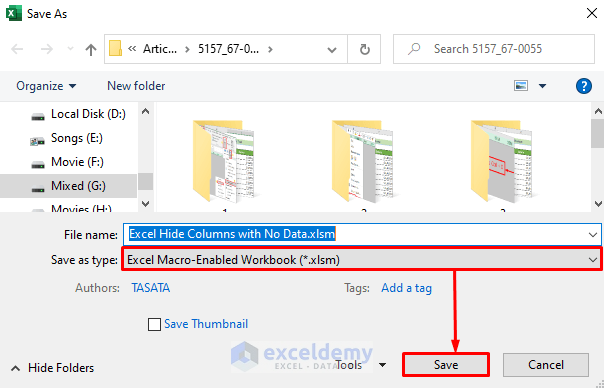
• In the Save As dialog box, select Save as type:
• Choose the .xlsm file and click Save.

• Go to the Developer tab >> Visual Basic.

• In Microsoft Visual Basic for Applications will open again.
• Select Sheet5 and click Run.

• In Macros, choose the Macro Name: and click Run.

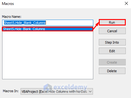
This is the output.

Read More: How to Hide and Unhide Columns in Excel

How to Unhide Hidden Columns?

Steps:

• Click the last column header (C here) and drag your mouse to the right.

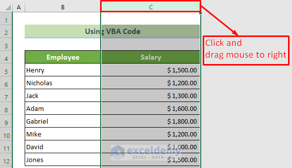
• Right-click .
• Choose Unhide.

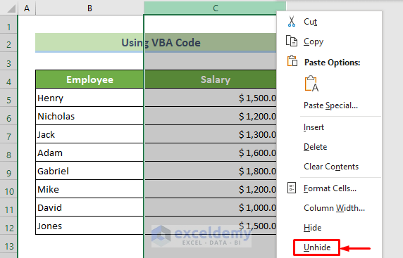
This is the output.

Download Practice Workbook

Download the practice workbook.

Related Articles

• How to Hide Extra Columns in Excel
• How to Unhide Columns in Excel All at Once
• Unhide Columns Is Not Working in Excel
• Unhide Columns in Excel Shortcut Not Working

<< Go Back to Hide Columns | Learn Excel