In this article, we are going to illustrate 7+ methods with examples to unhide columns in Excel. The feature to hide a column in Excel makes columns disappear from the display. You may have a lot of columns but don’t need to work with them all at once. To hide and unhide columns in Excel is important to make your worksheet look clean.
How to Unhide Columns in Excel: 8 Suitable Methods
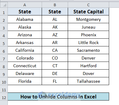
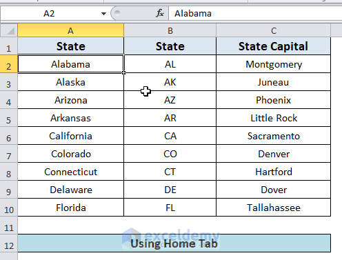
Our dataset is a list of the States in the U.S. their two-letter abbreviations, and their capital cities that are represented by Column A, Column B, and Column C consequently.
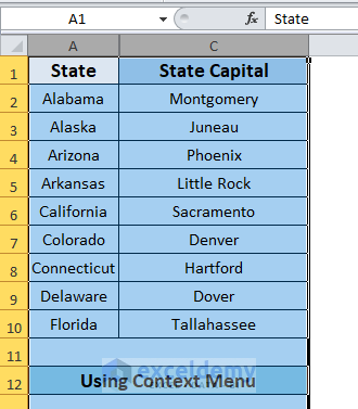
1. Unhide Columns in Excel Using Context Menu
The first method shows how to show hidden columns in Excel using the context menu. In our example dataset, we have got one of the three columns hidden (Column B). Let’s make it visible by using the context menu.
- Firstly, we have to select the columns (Column A and Column C) to the left and right of Column B.
- Then, we have to Right-click the mouse and choose Unhide.
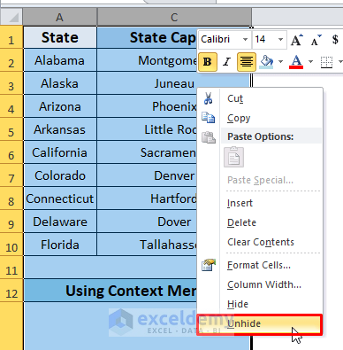
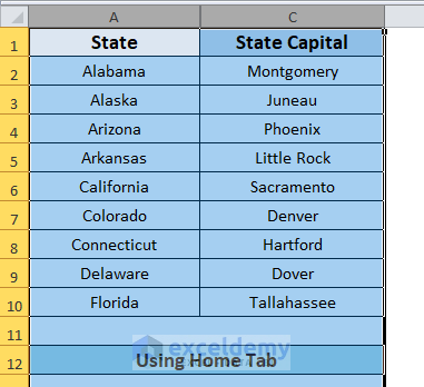
- Finally, we’ve got our hidden column revealed.

Read More: How to Hide Columns with Button in Excel
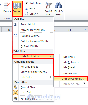
2. Show Hidden Columns with the Home Tab of Excel Ribbon
The Home Tab of Excel provides the option to hide and unhide columns. In this method, we are going to explore that option.
- At first, we need to select columns A to C.
- Then, from the Excel Ribbon:
- Select Home tab
- Click Format option
- From Visibility hover on the Hide & Unhide
- Finally, choose the Unhide Columns option
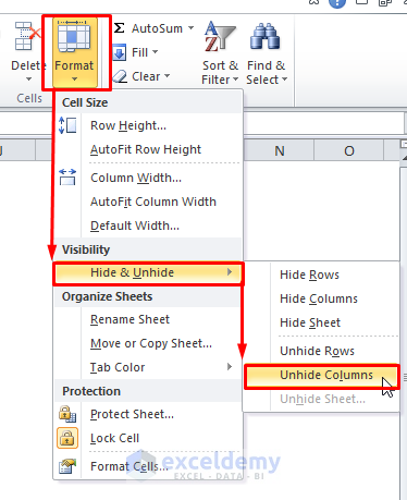
As a result, we’ll have our hidden column B unhidden.
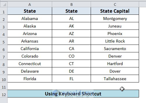
3. Keyboard Shortcut to Unhide Columns in Excel
Keyboard shortcuts can perform a task easily and quickly. Excel provides keyboard shortcuts to unhide columns. Let’s dive in:
- In the first step, we have to select the columns (Column A, Column C) to the left and right of the column (Column B) we want to unhide.
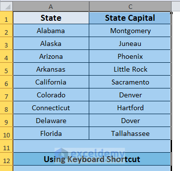
- Now, on your keyboard press Alt + H + O + L and see the output.
Read More: Hide Columns with No Data in Excel
4. Reveal Hidden Columns by Setting Column Width in Excel
The context menu (Right-Click Menu) has the option to define a column width that can be used to make hidden columns visible. In our dataset:
- After selecting columns A and C, right-click the mouse to pop up the context menu and, then click on Column Width.

- The above step will show up in the Column Width window. Put any desired value as we put 20, in this instance. At the end of the process, hit OK.
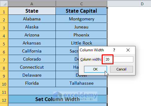
- Finally, the output shows Column B visible.

5. Use the Go To Command to Disclose Hidden Columns in Excel
In this example, we hide column A, the first column of the dataset. As a result, there is nothing to select to the left of the hidden column. So, we’ll use the Go To command to first select a cell of the hidden column and then reveal the whole column A.
- Press Ctrl + G to open up the Go To window. Put A2 in the Reference input box and hit OK. Now, cell A2 is selected in the worksheet although it is not visible.

- Now, from the Excel Ribbon:
-
- Select Home tab
- Click Format option
- From Visibility hover on the Hide & Unhide
- Finally, choose the Unhide Columns option
- The final result is here:

Read More: How to Hide Multiple Columns in Excel
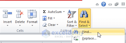
6. Use Find and Select to Show Hidden Columns in Excel
Using the Find & Select method, we can disclose a column in Excel. At first, we have to find and select a cell of that hidden column by using Find & Select. Using the same dataset, we have got column B as hidden. Let’s follow the guide:
- From the Home tab of the Excel Ribbon, click Find & Select and then choose Find.
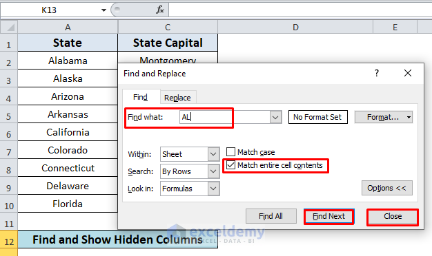
- In the Find and Replace window:
-
- Put a value (Here we put AL, the value of B2 Cell of the hidden column B) of any of the hidden column’s cells in the Find what input box
- Check Match entire cell contents option
- Click the Find Next button
- Then, Close the window.
This will get cell B2 of column B selected.
- Now, from the Excel Ribbon:
-
- Select Home tab
- Click Format option
- From Visibility hover on the Hide & Unhide
- Finally, choose the Unhide Columns option.
That’ll unhide the hidden column successfully.
7. Show Hidden Columns by Double Clicking the Hidden Column Indicator
- In Excel, when we hide a column it shows a double line indicator.
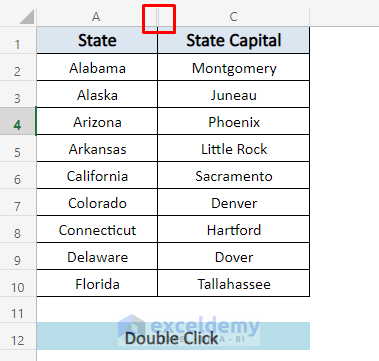
- Double-click the indicator; it’ll bring our hidden column into the light.

Read More: How to Hide Columns Without Right Click in Excel
8. VBA Code to Disclose Hidden Columns in Excel
Using simple VBA code is also an easy solution to unhide a hidden column in MS Excel. Let’s see how we can perform this:
- Go to the Developer tab and click the Visual Basic option.

- It would open up the Visual Basic editor. From here, create a new Module from the Insert tab option.

- Finally, we need to put the code and run it (F5).
Sub UnhideCols()

Columns.EntireColumn.Hidden = False
End Sub
Read More: How to Hide and Unhide Columns in Excel
Things to Remember
Hiding a column in Excel makes a column disappear from the view, that’s it. The hidden column still remains with all of its values. While sharing a file with editing enabled means someone can retrieve your hidden values using simple methods. So, don’t forget to lock your file before sharing.
Download Practice Book
Download this practice workbook to exercise while you are reading this article.
Conclusion
Now we know the methods to unhide columns, it would encourage you to take benefit of Excel’s hide and unhide feature more confidently. Any questions or suggestions don’t forget to put them in the comment box below.
Related Articles
- How to Hide Extra Columns in Excel
- How to Unhide Columns in Excel All at Once
- Unhide Columns Is Not Working in Excel
- Unhide Columns in Excel Shortcut Not Working
<< Go Back to Hide Columns | Columns in Excel | Learn Excel
Get FREE Advanced Excel Exercises with Solutions!
