How to Highlight Duplicates in Two Columns Using Excel Formula

If you are looking for some special tricks to highlight duplicates in two columns using the Excel formula, you’ve come to the right place. In Microsoft Excel, there are numerous ways to highlight duplicates in two columns. In this article, we’ll discuss four methods to highlight duplicates in two columns using the Excel formula. Let’s follow the complete guide to learn all of this.

Download Practice Workbook

Download this practice workbook to exercise while you are reading this article.

4 Ways to Highlight Duplicates in Two Columns Using Excel Formula

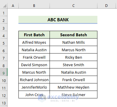
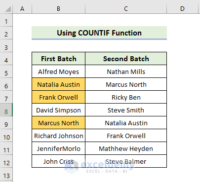
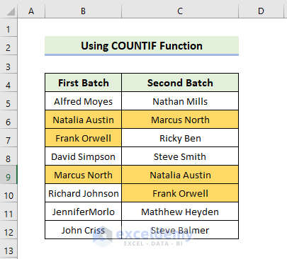
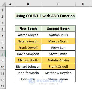
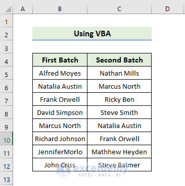
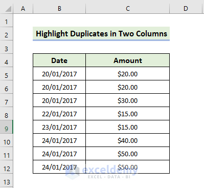
Here, we have a dataset containing the names of the first and second batches of employees of ABC bank. The main objective is to identify duplicate names of the first and second batches of the ABC bank.

In the following section, we will use 4 methods to highlight duplicates in two columns using Excel formula.

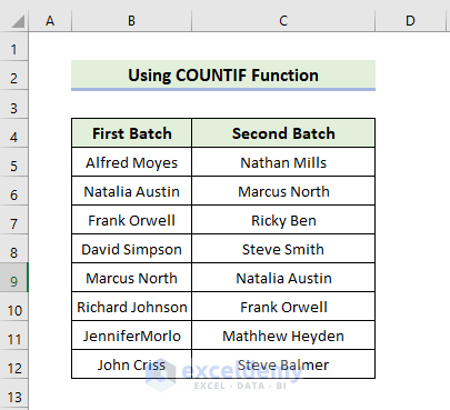
1. Using COUNTIF Function to Highlight Duplicates in Two Columns

You have to follow the following rules to highlight duplicates in two columns by using the COUNTIF function.

📌 Steps:

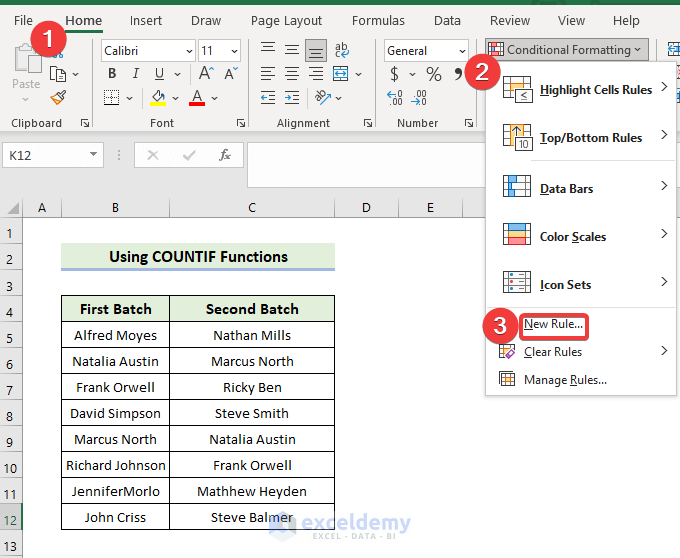
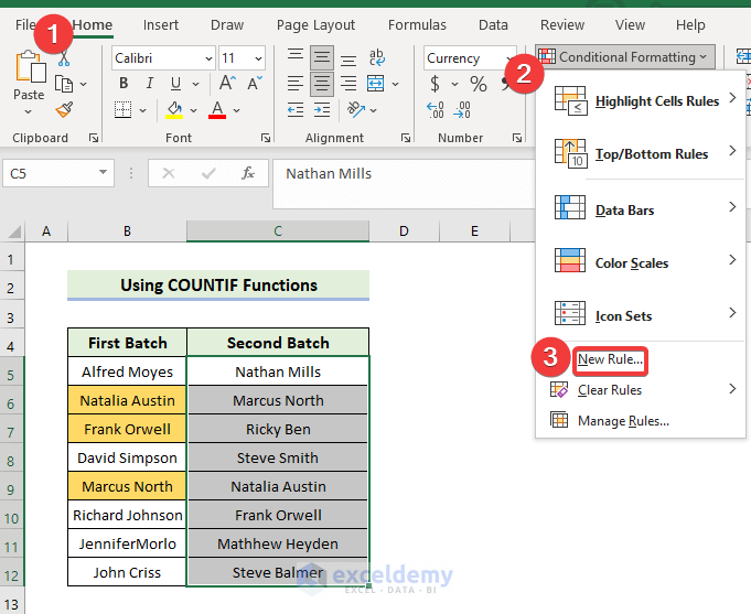
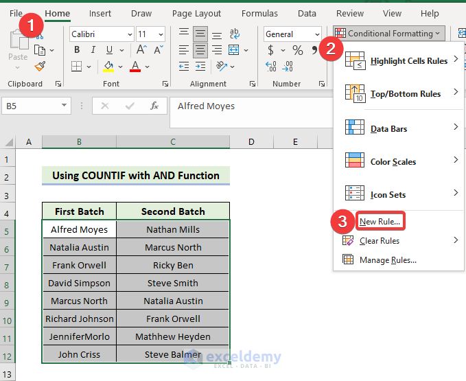
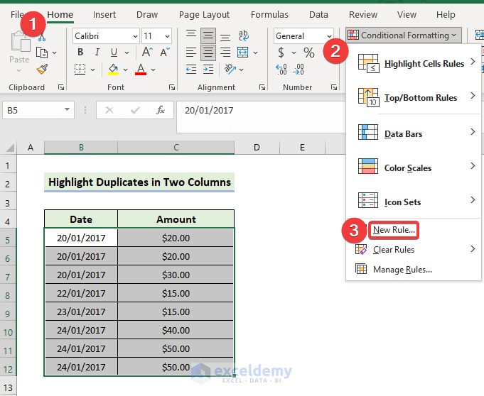
• Select the first batch column, go to the Home tab, and select the Conditional Formatting From the options, select New Rule.

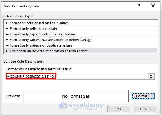
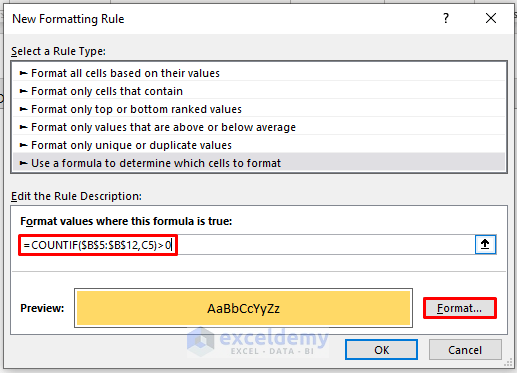
• When the New Formatting Rule dialogue box appears, select Use a formula to determine which cells to format.
• Next, in the Format values where this formula is true box, you have to insert the following formula:

• Here, $C$5:$C$12 is the second batch column and B5 is the first cell of the first batch column.

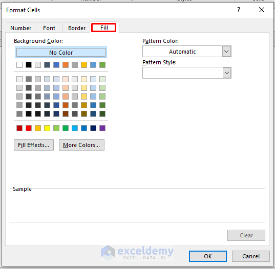
• Now, click on Format, when the Format cells dialogue box appears, you have to fill your desired color by selecting the Fill Click on OK.

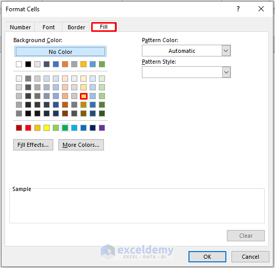
Finally, you will get the following output:

• Now you have to select the first batch column, go to the Home tab, and select the Conditional Formatting tool. From the options, select New Rule.

• When the New Formatting Rule dialogue box appears, select Use a formula to determine which cells to format.
• Next, in the Format values where this formula is true box, you have to insert the following formula:

• Here, $B$5:$B$12 is the first batch column and C5 is the first cell of the second batch column.

• Now, click on Format, when the Format cells dialogue box appears, you have to fill your desired color by selecting the Fill Click on OK.

Finally, you will be able to highlight duplicates in two columns using Excel formula like the following:

Read More: How to Highlight Duplicates in Excel (6 Easy Ways)

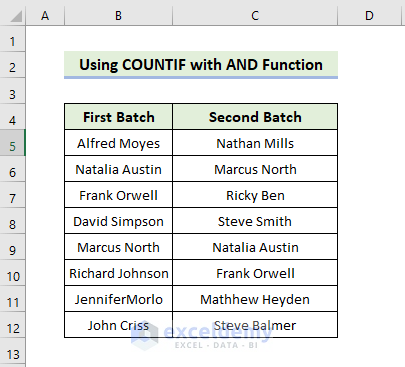
2. Combining COUNTIF with AND Function to Highlight Duplicates

Here is another method to highlight duplicates in two columns by using the AND function and the COUNTIF function. You have to follow the following steps to do this:

📌 Steps:

• Firstly, select the first batch and second batch column, go to the Home tab, and select the Conditional Formatting tool. From the options, select New Rule.

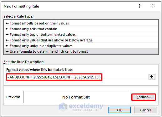
• When the New Formatting Rule dialogue box appears, select Use a formula to determine which cells to format.
• Next, in the Format values where this formula is true box, you have to insert the following formula:

• Here, $B$5:$B$12IS is the first batch column, $C$5:$C$12 is the second batch column and B5 is the first cell of the first batch column.
• Here, the COUNTIF function counts the number of the cells within a range that meet the given condition, and the AND function check whether all arguments are true, and returns true if all arguments are true.

• Now, click on Format, when the Format cells dialogue box appears, you have to fill your desired color by selecting the Fill Click on OK.

Finally, you will get the following output.

Read More: How to Highlight Duplicates in Multiple Columns in Excel (4 Ways)

3. Using VBA to Highlight Duplicates

You have to follow the following steps to highlight duplicates in two columns.

📌 Steps:

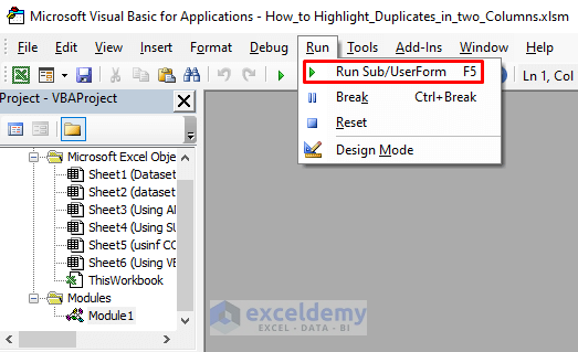
• Firstly, press ALT+F11 or you have to go to the tab Developer, select Visual Basic to open Visual Basic Editor, and click Insert, select

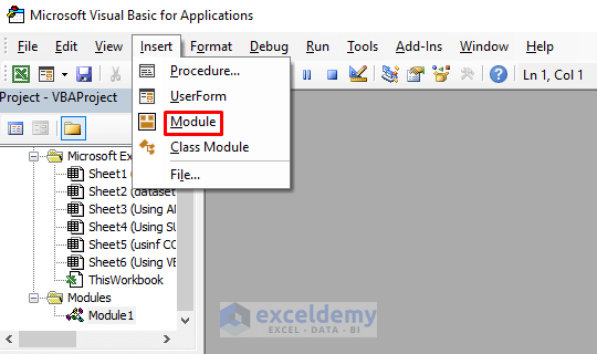
• Next, you have to type the following code:

Sub highlight_duplicate()
Dim range_1 As Range, range_2 As Range, rng_1 As Range, rng_2 As Range, out_range As Range
xTitleId = "Using VBA "
Set range_1 = Application.Selection
Set range_1 = Application.InputBox("range_1:", xTitleId, range_1.Address, Type:=8)
Set range_2 = Application.InputBox("range_2:", xTitleId, Type:=8)
Application.ScreenUpdating = False
For Each rng_1 In range_1
 xValue = rng_1.Value
 For Each rng_2 In range_2
  If xValue = rng_2.Value Then
   If out_range Is Nothing Then
    Set out_range = rng_1
   Else
   Set out_range = Application.Union(out_range, rng_1)
   End If
  End If
 Next
Next
out_range.Select
Application.ScreenUpdating = True
End Sub

• Now, press F5 or select Run, and click on Run Sub/UserFrom.

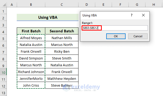
• Now, select the first batch column as Range 1.

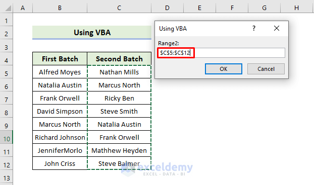
• Next, select the second batch column as Range 2.

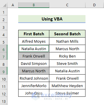
Finally, you will get the following output.

Read More: [Fix:] Highlight Duplicates in Excel Not Working

4. SUMPRODUCT and COUNTIF Functions to Highlight Duplicates in Two Columns

Here is another method to highlight duplicates by using the SUMPRODUCT function and the COUNTIF function. You have to follow the following steps to do this:

📌 Steps:

• Firstly, select the first batch and second batch column, go to the Home tab, and select the Conditional Formatting tool. From the options, select New Rule.

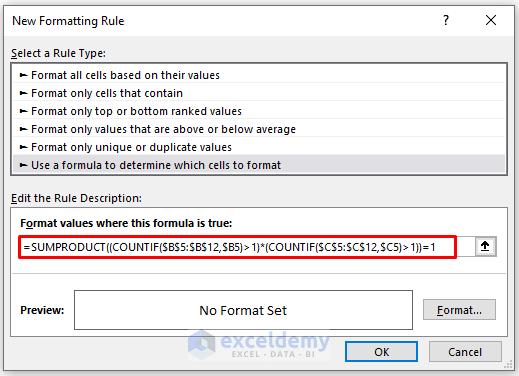
• When the New Formatting Rule dialogue box appears, select Use a formula to determine which cells to format.
• Next, in the Format values where this formula is true box, you have to insert the following formula:

• Now, click on Format, when the Format cells dialogue box appears, you have to fill your desired color by selecting the Fill Click on OK.

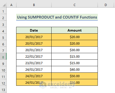
Finally, you will get the following output:

Read More: How to Highlight Duplicates but Keep One in Excel (4 Methods)

💬 Things to Remember

✎ If you are using the combined large formula, you should carefully use the parentheses.

Conclusion

That’s the end of today’s session. I strongly believe that from now you may highlight duplicates in two columns. If you have any queries or recommendations, please share them in the comments section below.

Don’t forget to check our website Exceldemy.com for various Excel-related problems and solutions. Keep learning new methods and keep growing!

Related Articles

• How to Highlight Duplicate Rows in Excel (3 Ways)
• Highlight Duplicates across Multiple Worksheets in Excel (3 Formulas)
• How to Highlight Duplicates in Excel with Different Colors (2 Ways)
• Highlight Cells If There Are More Than 3 Duplicates in Excel (3 Examples)