Method 1. Highlighting Duplicate Rows in One Column with the Built-in Rule in Excel
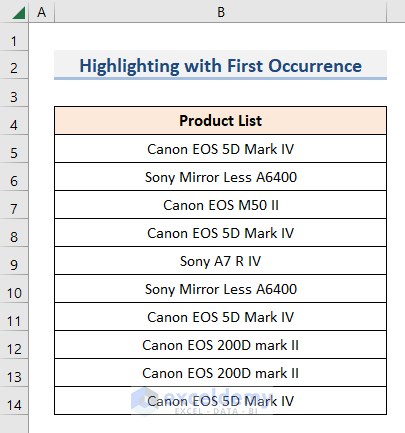
1.1. Including First Occurrence
This is the sample dataset.
- Select the range B5:B14.
- Go to the Home tab and click Conditional Formatting in the Style section.
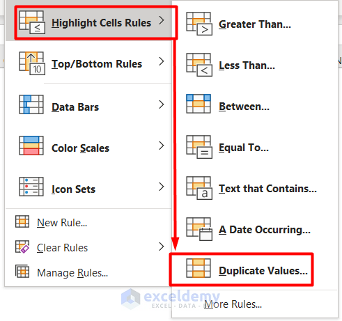
- Click Highlight Cell Rules.
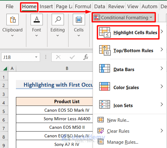
- Select Duplicate Values.
- In the Duplicate Values dialog box, choose Duplicate.
- Select a format. Red Text, here.
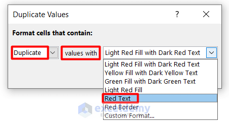
- Click OK to highlight duplicate rows .
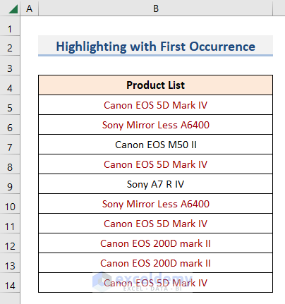
1.2. Excluding First Occurrence
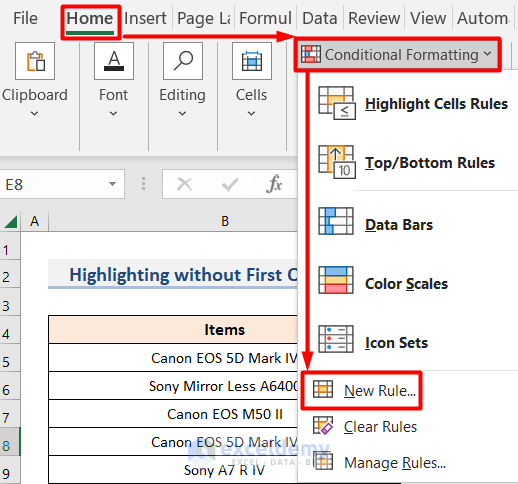
- Select the range B5:B14.
- Choose Home > Conditional Formatting > New Rule.
- In New Formatting Rule, select Use a Formula to Determine Which Cells to Format.
- Enter this formula Format Values Where This Formula is True.
=COUNTIF($B$5:$B5,$B5)>1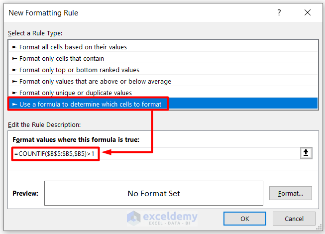
The COUNTIF function counts cells in the $B$5:$B5 range based on the criteria in $B5.
- Click Format to select a format style for the highlighted rows.
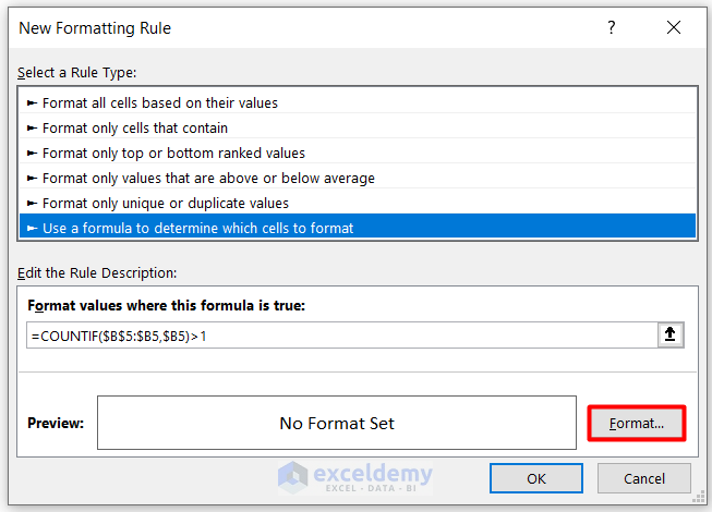
- Here, Bold as the Font style and Red as the Color.
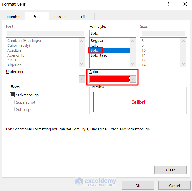
- Click OK twice.
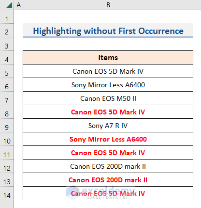
The highlighted duplicate rows are showcased without the first occurrence.
Read More: How to Highlight Duplicates but Keep One in Excel
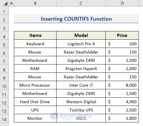
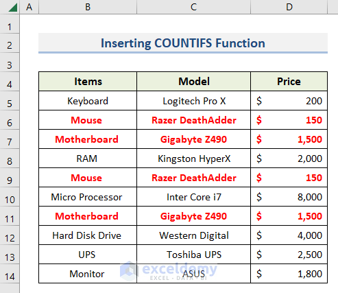
Method 2. Inserting the COUNTIFS Function to Highlight Duplicate Rows in Excel
This is the dataset.
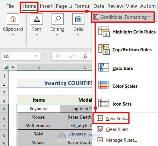
- Select the dataset and click Home > Conditional Formatting > New Rule.
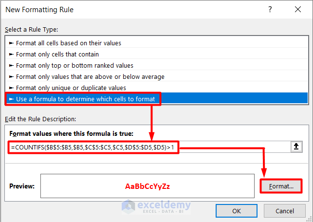
- In New Formatting Rule, select Use a Formula to Determine Which Cells to Format.
- Enter this formula in Format Values Where This Formula is True.
=COUNTIFS($B$5:$B$14,$B5,$C$5:$C$14,$C5,$D$5:$D$14,$D5)>1- Select Format.

The COUNTIFS function applies the criteria ($B5, $C5, $D5) across the $B$5:$B$14, $C$5:$C$14 and $D$5:$D$14 ranges and counts cells that meet the criteria.
- Click OK.
This is the output.
- Use this formula to highlight duplicate rows without the first occurrence.
=COUNTIFS($B$5:$B5,$B5,$C$5:$C5,$C5,$D$5:$D5,$D5)>1- Select Format and click OK.
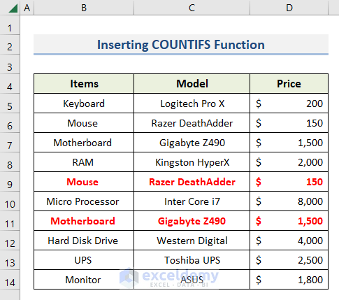
The duplicate rows are highlighted without the first occurrence.
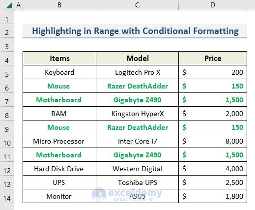
Method 3 – Highlighting Duplicate Rows in a Range Using the Excel Conditional Formatting
- Select the dataset and click Home > Conditional Formatting > New Rule.
- Enter this formula in Format Values Where This Formula is True.
=COUNTIFS($B$5:$D$14,B5)>1- Select Format and click OK.
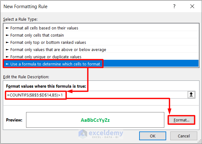
Here the range is $B$5:$D$14 and the criteria is B5.
Duplicate rows are highlighted in a range.
- To highlight the duplicate rows in a range without the first occurrence, enter this formula in Format Values Where This Formula is True.
=COUNTIFS($B$5:$B5,$B5)>1- Select Format and click OK twice.
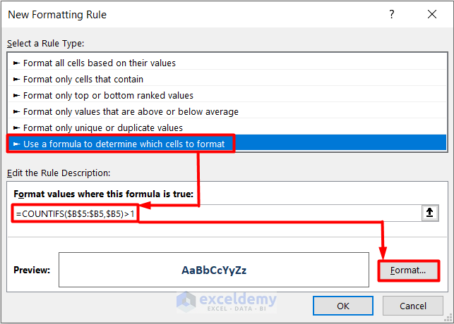
Here, the range and criteria are $B$5:$B5 and $B5.
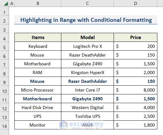
This is the output.
Download Practice Workbook
Download this sheet to practice.
Related Articles
- Highlight Cells If There Are More Than 3 Duplicates in Excel
- How to Highlight Duplicates in Excel with Different Colors
- How to Highlight Duplicates in Two Columns in Excel
- How to Highlight Duplicates in Two Columns Using Excel Formula
- How to Highlight Duplicates in Multiple Columns in Excel
- Highlight Duplicates across Multiple Worksheets in Excel
- [Fix:] Highlight Duplicates in Excel Not Working
<< Go Back to Highlight Duplicates in Excel | Learn Excel
Get FREE Advanced Excel Exercises with Solutions!
