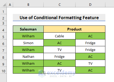
Example 1 – Using the Conditional Formatting Feature to Highlight Cells from Multiple Rows If There Are More Than 3 Duplicates
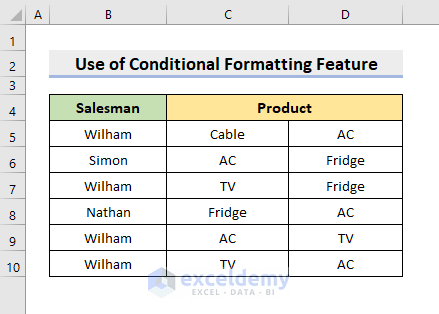
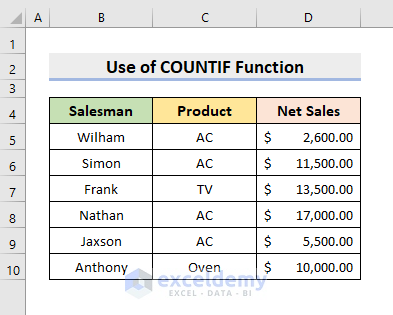
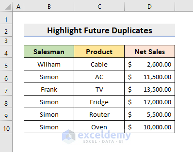
This is the sample dataset.
STEPS:
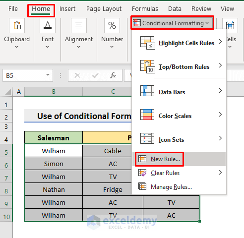
- Select B5:D10.
- In the Home tab, go to Conditional Formatting and select New Rule.
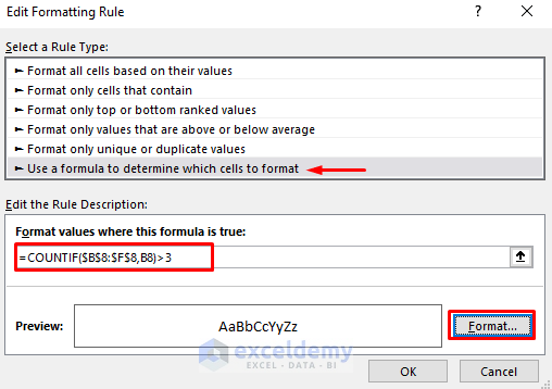
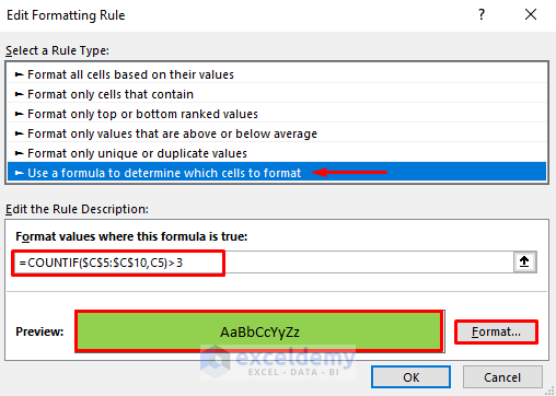
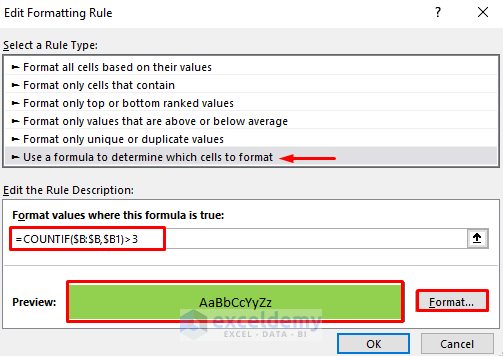
- In the New Formatting Rule dialog box, select the 6th Rule Type (as shown below in 1).
- In Format values where this formula is true, enter the formula:
=COUNTIF($B$5:$D$10, B5)>3- Click Format.
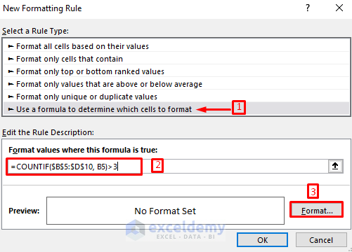
The COUNTIF function counts the total number of cells based on criteria. $B$5:$D$10 is the criteria range and B5 is the criteria. It will format the cells which appear more than 3 times.
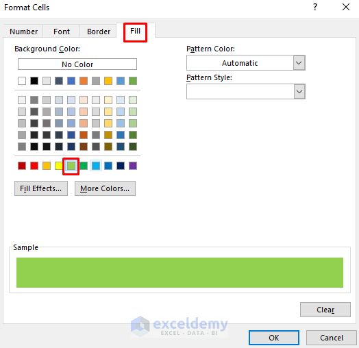
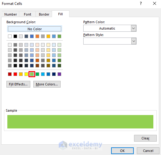
- In the Format Cells dialog box, select Fill.
- Choose a color to highlight the cells, here Green.
- Click OK.
- Click OK.
The cells which appear more than 3 times are highlighted in Green.
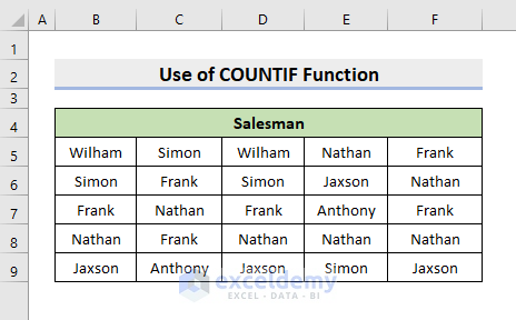
Example 2 – Highlight Cells When There Are More Than 3 Duplicates with the Excel COUNTIF Function
2.1 From Individual Rows
Consider the 8th row.
STEPS:
- Select B8:F8.
- Go to Home ➤ Conditional Formatting ➤ New Rule.
- In the dialog box, select the 6th Rule Type.
- Enter the formula:
=COUNTIF($B$8:$F$8,B8)>3- Click Format.
- In the Format Cells dialog box, select Fill.
- Choose a color to highlight the cells, here Green.
- Click OK.
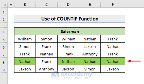
You’ll see the highlighted cells in the 8th row.
2.2 From Individual Columns
Consider column C.
STEPS:
- Select C5:C10.
- Go to Home ➤ Conditional Formatting ➤ New Rule.
- In the dialog box, select the 6th Rule Type.
- Enter the formula:
=COUNTIF($C$5:$C$10,C5)>3- Choose Green to highlight the cells and click OK.
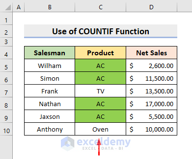
This is the output.
Read More: How to Highlight Duplicates in Two Columns Using Excel Formula
Example 3 – Highlight Future Duplicates in the Selected Range
Consider column B.
STEPS:
- Select column B.
- Go to Home ➤ Conditional Formatting ➤ New Rule.
- In the dialog box, select the 6th Rule Type.
- In Format values where this formula is true, enter the formula:
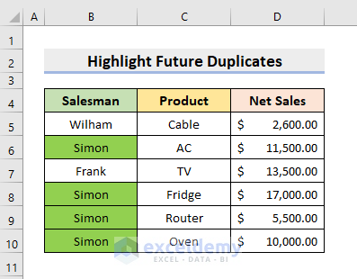
=COUNTIF($B:$B,$B1)>3- Choose Green to highlight the cells and click OK.
This is the output.
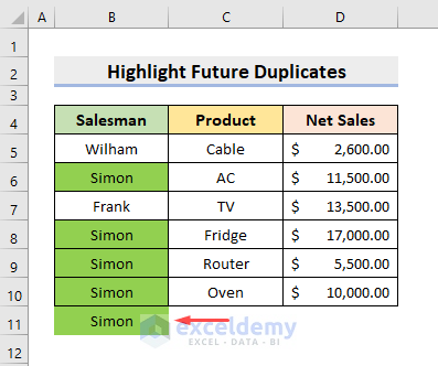
- Enter Simon in B11 and press Enter.
- The cell is highlighted.
Read More: Highlight Duplicates across Multiple Worksheets in Excel
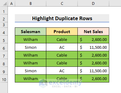
Highlight Rows If There Are More Than 3 Duplicates in Excel
The 5th, 7th, 8th and 10th rows are identical.

STEPS:
- Select B5:D10.
- Go to Home ➤ Conditional Formatting ➤ New Rule.
- In the dialog box, select the 6th Rule Type.
- Enter the formula:
=COUNTIFS($B$5:$B$10,$B5,$C$5:$C$10,$C5,$D$5:$D$10,$D5)>3- Choose Green to highlight the cells and click OK.
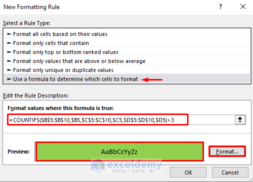
There are 3 ranges in the argument section: $B$5:$B$10, $C$5:$C$10, and $D$5:$D$10. The criteria are $B5, $C5, and $D5. The formula will format cells with more than 3 duplicates.
This is the output.
Download Practice Workbook
Download the following workbook.
Related Articles
- How to Highlight Duplicates but Keep One in Excel
- How to Highlight Duplicates in Excel with Different Colors
- How to Highlight Duplicates in Two Columns in Excel
- How to Highlight Duplicates in Multiple Columns in Excel
- How to Highlight Duplicate Rows in Excel
- [Fix:] Highlight Duplicates in Excel Not Working
<< Go Back to Duplicates in Excel | Learn Excel
Get FREE Advanced Excel Exercises with Solutions!

I keep getting “Youve entered too few arguments for this function” and i cannot get around it 🙁
Hello Ruby,
Greetings from our website. You have encountered a warning message from the Microsoft Excel window. The error message “You’ve entered too few arguments for this function” means not providing enough arguments or inputs for a particular formula or function to work correctly. To resolve this error, check the formula or function you’re using and ensure you’ve provided all the required arguments.
This article explains how we can highlight cells with more than three duplicates. But, if you need help understanding this post, you can follow another article on the ExcelDemy website link given below.
How to Do Conditional Formatting in Excel [Ultimate Guide]
Later go through this article to better understand and highlight if there are more than three duplicates. Good luck.
Regards
Lutfor Rahman Shimanto