Today I’ll show how to highlight duplicates in two columns in Excel with easy examples and proper illustrations.
Highlight Duplicates in Two Columns in Excel: 2 Examples
1. Highlight Duplicates in Two Columns of the Same Row
Here we’ve got a data set with the Names of some employees, and their Starting and Present salaries of a company called Rennata Group.
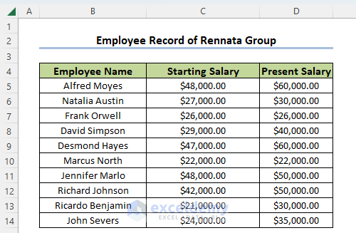
Our objective is to highlight the employees whose salaries didn’t increase, which means the starting salary and the present salary are the same.
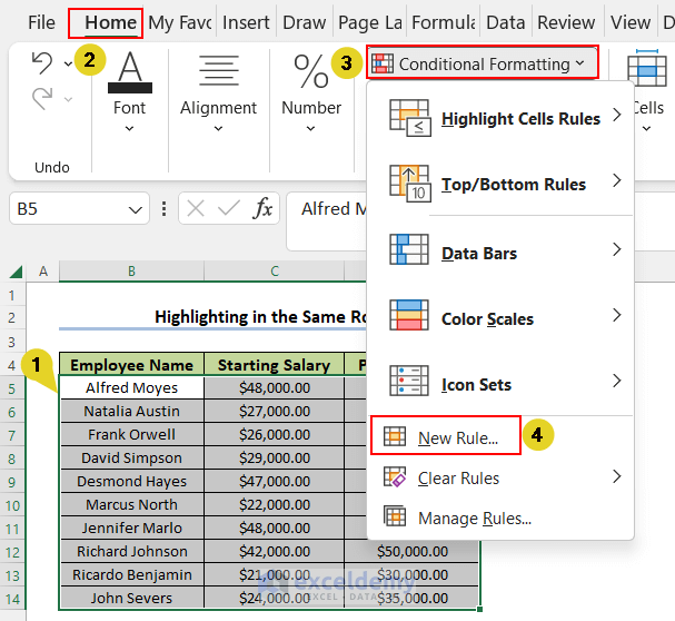
- Select the whole data set (Without the Column Headers).
- Go to the Home>Conditional Formatting tool in the Excel toolbar.
- Click on the drop-down menu associated with Conditional Formatting.
- From the options available, select New Rule.
- You will get a dialogue box called New Formatting Rule.
- Select Use a formula to determine which cells to format.
- Then in the Format values where this formula is true box, insert the following formula:
=$C5=$D5
Here $C5 and $D5 are the first cells of my two columns. You use your one. But don’t change the Mixed Cell Reference as presented.
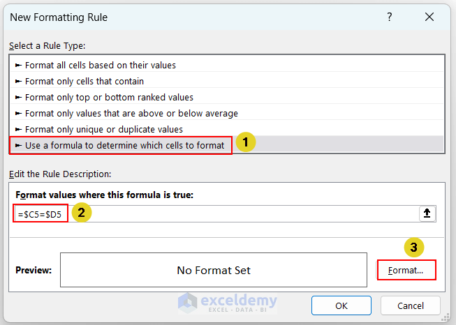
- Click on Format.
- You will get the Format Cells dialogue box. Choose any format that you like to highlight the cells with duplicate values.
- Here I have selected Yellow color under the option Fill. This will fill the cell background in yellow.

- Click on OK. You will come back to the New Formatting Rule box.
- Again click on OK. You will find the rows that have the same joining and present salaries have been highlighted in yellow.

Read More: How to Highlight Duplicate Rows in Excel
2. Highlight Duplicates in Two Columns of Different Rows
Here we’ve got another data set with the Candidates of two weeks for an interview in Rennata Group.

Today, our objective is to find out if any candidate is mistakenly put into both weeks or not.
We will highlight the names that appear in both weeks.
🔀 Steps:
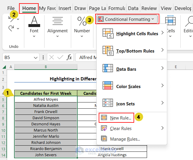
- Select the first column (Except the Column Header)
- Then go to the Home > Conditional Formatting tool in Excel Toolbar.
- Click on the drop-down menu associated with Conditional Formatting.
- Then from the options available, select New Rule.
- You will get a dialogue box called New Formatting Rule.
- Select Use a formula to determine which cells to format.
- Then in the Format values where this formula is true box, insert the formula below:
=COUNTIF($C$5:$C$14,B5)>0
- Here $C$5:$C$14 is my second column. You use your one.
- But don’t change the Absolute Cell Reference as presented.
- B5 is the first cell of my first column. You use your one.
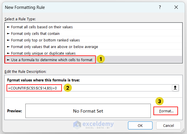
- Click on Format. You will get the Format Cells dialogue box.
- Choose any format that you like to highlight the cells with duplicate values. Here I have selected Yellow color under the option Fill. This will fill the cell background in yellow.

- Click on OK. You will come back to the New Formatting Rule box.
- Then again click on OK. You will find the names in your first column that have duplicates in the second column highlighted in yellow.

We have highlighted the names in the first week that appear in the second week.
- And to highlight them in the second week also, repeat the same procedure.
- This time, the formula will be:
=COUNTIF($B$5:$B$14,C5)>0
- Here $B$4:$B$13 is my first column. You use your one.
- But don’t change the Absolute Cell Reference as presented.
- C4 is the first cell of my second column. You use your one.
- The output will be as follows.

Read More: How to Highlight Duplicates in Excel with Different Colors
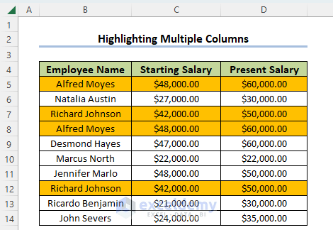
How to Highlight Duplicates in Multiple Columns in Excel
Now, what if you have data in more than two columns and still have to check for duplicate values? Here comes the solution. In this section, we will discuss how to highlight duplicates in multiple columns.
Here, the following dataset will be used.

- Follow the same procedure described in Example 1. Use the following formula in this case.
=COUNTIFS($B$5:$B$14,$B5,$C$5:$C$14,$C5,$D$5:$D$14,$D5)>1- If you have more columns, for example, more data in column E, then add $E$5:$E$14,$E$5 in this formula.
- The final output will be as follows. So you can now easily track duplicates in multiple columns in Excel.
Download Practice Workbook
You can download the following workbook for your practice while reading this article.
Conclusion
Using this method, you can highlight duplicates in two columns in Excel. Do you know any other method? Or do you have any questions? Feel free to ask us.
Related Articles
- How to Highlight Duplicates but Keep One in Excel
- Highlight Cells If There Are More Than 3 Duplicates in Excel
- How to Highlight Duplicates in Two Columns Using Excel Formula
- Highlight Duplicates across Multiple Worksheets in Excel
- [Fix:] Highlight Duplicates in Excel Not Working
<< Go Back to Highlight Duplicates in Excel | Duplicates in Excel | Learn Excel
Get FREE Advanced Excel Exercises with Solutions!
