Method 1 – Use COUNTIF Function to Highlight Matches Across Excel Worksheets
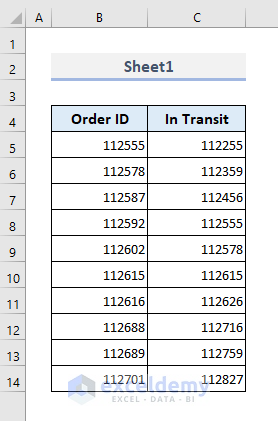
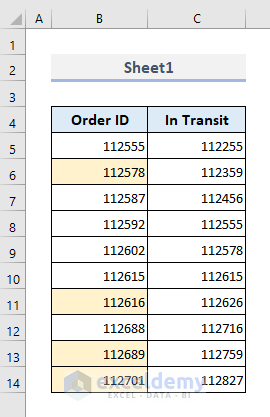
The following picture represents a worksheet named Sheet1. It contains two columns. One showing random order IDs (left) and IDs that are in transit (right).
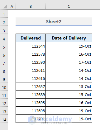
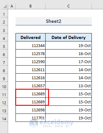
In Sheet2, the left column shows the IDs of delivered orders and the right column shows the corresponding delivery dates.
We’ll look for all the duplicates of order IDs across Sheet1 and Sheet2. The matched order IDs in Sheet1 will be highlighted with a selected color.
Step 1:
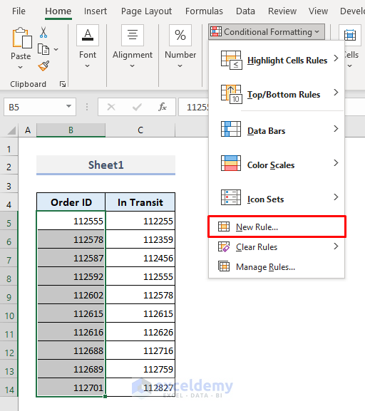
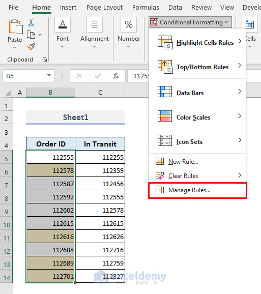
➤ From Sheet1, select the range of cells where the duplicate values will be highlighted.
➤ Go to Home and select the New Rule command from the Conditional Formatting drop-down menu.
A dialogue box named ‘New Formatting Rule’ will appear.
Step 2:
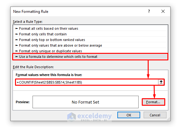
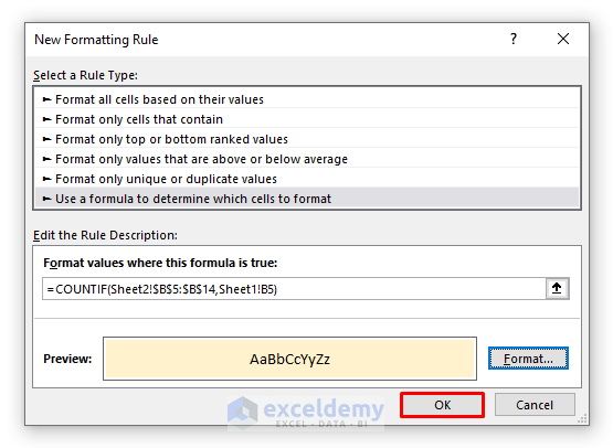
➤ From the Rule Type options, select ‘Use a formula to determine within cells to format’.
➤ Copy the following formula to the formula box:
=COUNTIF(Sheet2!$B$5:$B$14, Sheet1!B5)➤ Press Format.
Step 3:
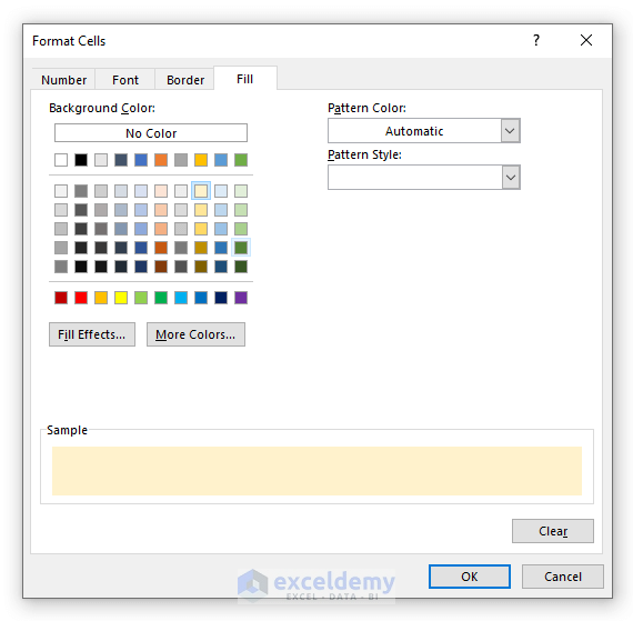
➤ In the Format Cells window, select a color for highlighting the duplicates.
➤ Press OK.
Step 4:
➤ You’ll find the preview of the formatted cell with text in the New Formatting Rule dialog box.
➤ Press OK.
Finally in Sheet1, you’ll see the highlighted cells with the order IDs that are also present in Sheet2.

Highlight Multiple Duplicates Across Two Worksheets
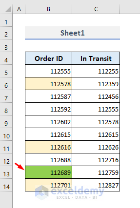
Let’s assume we have multiple duplicates for an order ID in Sheet2. In Sheet1, the corresponding order ID will be highlighted with another color or cell format.
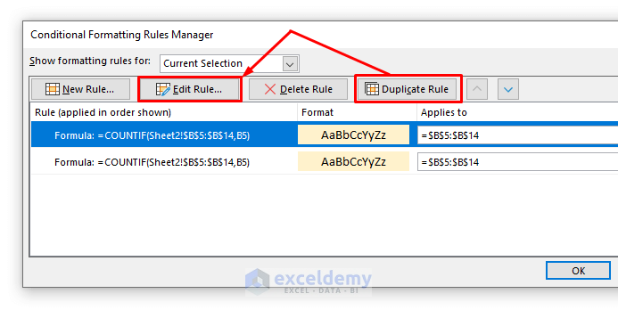
Step 1:
➤ In Sheet1, select the range of cells for the order IDs again.
➤ Go to Home and choose the Manage Rules command from the Conditional Formatting drop-down menu.
A dialog box named Conditional Formatting Rules Manager will appear.
Step 2:
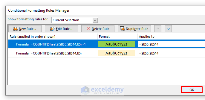
➤ Click on the option ‘Duplicate Rule’. This will create a duplicate of your previously defined rule.
➤ Select Edit Rule and the Edit Formatting Rule window will show up.
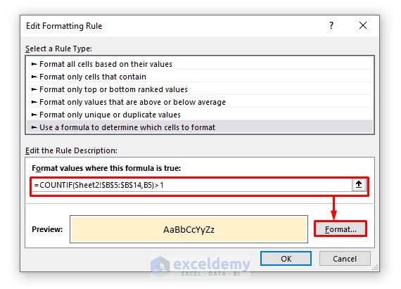
Step 3:
➤ In the formula box of the Rule Description, enable editing and add “>1” at the end of the formula.
➤ Click on the Format option.
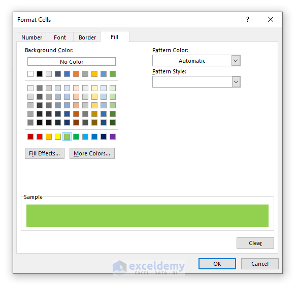
Step 4:
➤ Select a different color for the second formatting rule.
➤ Press OK.
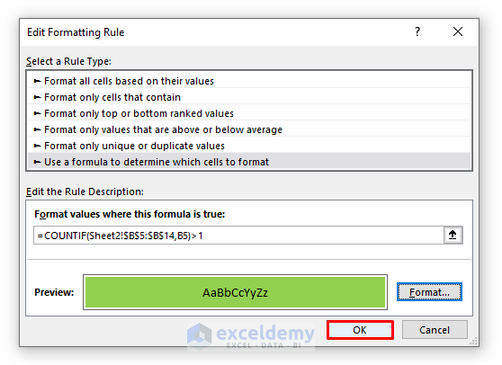
Step 5:
➤ You’ll be shown a preview of the second formatting rule. Click OK again.
Step 6:
➤ In the Conditional Formatting Rules Manager dialog box, the second rule is embedded now.
➤ Press OK for the last time and you’re done.
Like in the following screenshot, you’ll find Cell B13 highlighted with another color since this cell contains an order ID that is present multiple times in Sheet2.
Method 2 – Insert ISNUMBER Function to Find Duplicates across Multiple Worksheets in Excel
We can also combine the ISNUMBER and MATCH functions to find the duplicates or matches across two Excel worksheets. The MATCH function returns the relative position of an item in an array that matches a specified value in a specified order. And the ISNUMBER function checks whether a value is a number or not.
The required formula in the Rule Description box is:
=ISNUMBER(MATCH(B5, Sheet2!$B$5:$B$14,0))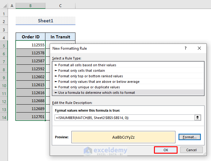
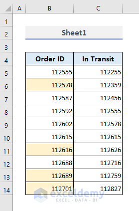
We’ll get the following result:
3. Apply the VLOOKUP Function to Highlight Duplicate Rows across Multiple Worksheets
The required formula with the VLOOKUP function in the Rule Box is:
=VLOOKUP(B5,Sheet2!B5:C14,,FALSE)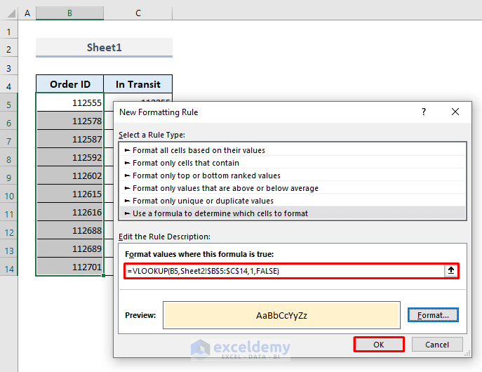
And the following picture shows the highlighted cells where the application of the VLOOKUP function has returned valid outputs.
Download Practice Workbook
You can download the Excel workbook that we’ve used to prepare this article.
Related Readings
- How to Highlight Duplicates but Keep One in Excel
- Highlight Cells If There Are More Than 3 Duplicates in Excel
- How to Highlight Duplicates in Excel with Different Colors
- How to Highlight Duplicates in Two Columns in Excel
- How to Highlight Duplicates in Two Columns Using Excel Formula
- How to Highlight Duplicates in Multiple Columns in Excel
- How to Highlight Duplicate Rows in Excel
- [Fix:] Highlight Duplicates in Excel Not Working
<< Go Back to Highlight Duplicates in Excel | Learn Excel
Get FREE Advanced Excel Exercises with Solutions!

Using only the COUNTIF formula, I’m trying to color fill the cells of sheet 1 (tab identified as “EBU Engines_APUs”), column B, when duplicates are identified in sheet 2 (tab identified as “Leased Parts”), column A. My formula is as follows:
=COUNTIF(‘Leased Parts’!$A:$A,$B:$B)
Although I don’t receive any errors, it’s simply not working. Nothing changes despite having duplicates in sheet 2.
Any assistance would be greatly appreciated! Thanks in advance.
Hello Keith Shelly
Thanks for visiting our blog and sharing your problem with such clarity. Instead of the current formula, you can try the following formula:
=COUNTIF('Leased Parts'!$A:$A, $B1)Hopefully, you have found the idea helpful. I have attached the solution workbook; good luck.
DOWNLOAD SOLUTION WORKBOOK
Regards
Lutfor Rahman Shimanto
ExcelDemy