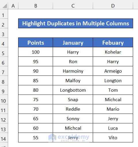
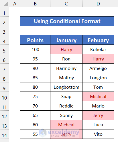
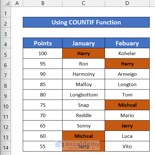
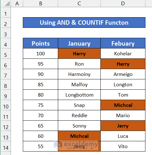
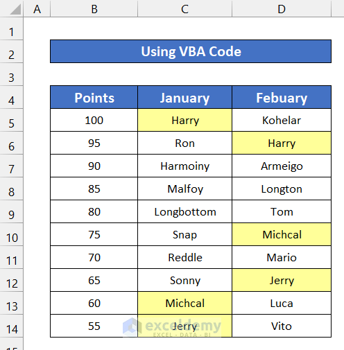
Let’s consider a dataset of 10 employees of a company. The point scale of this company is in column B. Their performance results for 2 months, January and February, are also shown in column C and column D. We will try to find out the employees’ names who are listed in both months with their excellent performance. Our dataset is in the range of cells B4:D14.
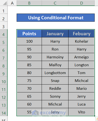
Method 1 – Using Conditional Formatting to Highlight Duplicates in Multiple Columns in Excel
Steps:
- Select the entire range of cells B4:D14.
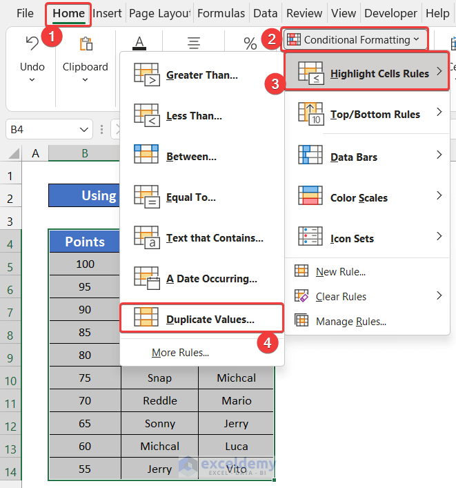
- In the Home tab, select Conditional Formatting.
- Select Highlight Cell Values and go to Duplicate values.
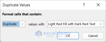
- A dialog box titled Duplicate Values will appear.
- Keep the first small box as Duplicate and choose the highlighting pattern. In our case, we chose the default Light Red with Dark Red Text option.
- Click the OK button.
- You will see the duplicate values get the selected highlight color.
Read More: Highlight Cells If There Are More Than 3 Duplicates in Excel
Method 2 – Inserting the Excel COUNTIF Function to Highlight Duplicates in Multiple Columns
Steps:
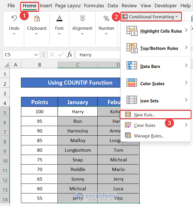
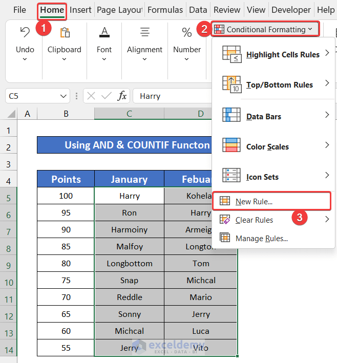
- Select the entire range of cells C5:D14.
- In the Home tab, select Conditional Formatting and pick New Rule.
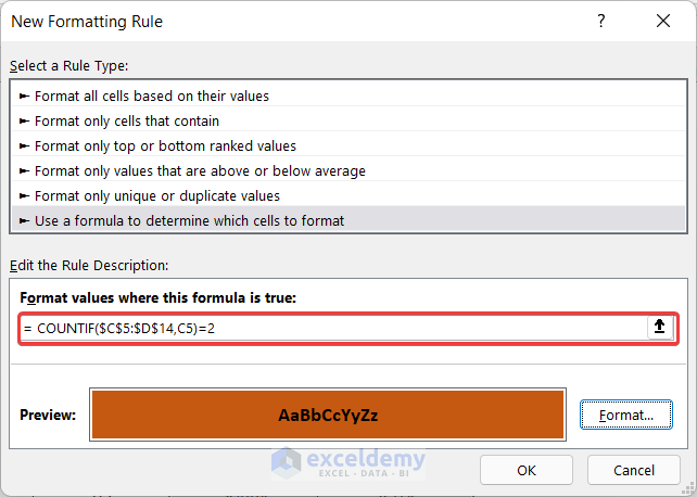
- A dialog box titled New Formatting Rule dialog box will appear.
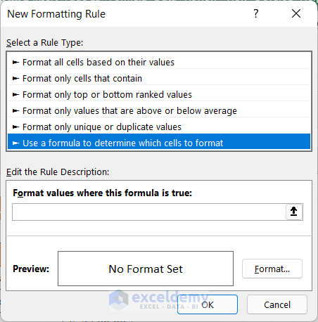
- Select the Use a formula to determine which cells to format option.
- Copy the following formula into the empty box below Format values where this formula is true.
=COUNTIF($C$5:$D$14,C5)=2
- Select the Format option.
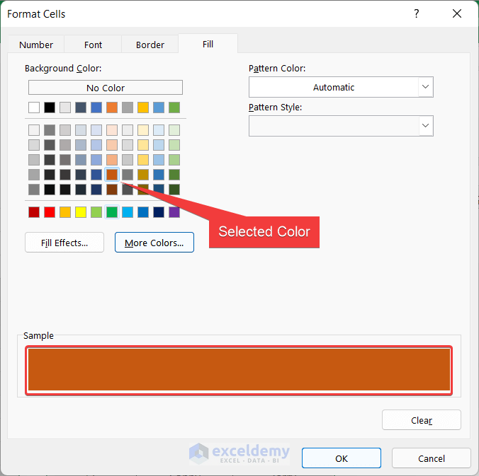
- Another dialog box called Format Cells will appear.
- Choose your highlighting pattern. We went to the Font tab and chose the Bold option.
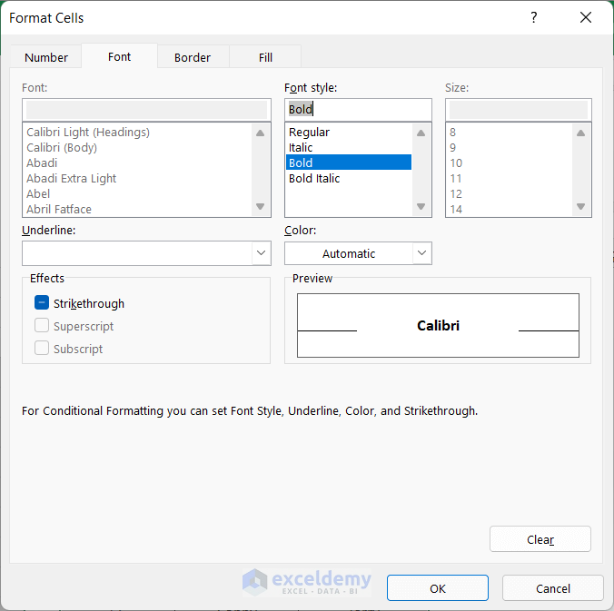
- In the Fill tab, you can select the cell fill color.
- Click OK to close the Format Cells dialog box.
- Click OK to close the New Formatting Rule box.
- You will see that the duplicate values of columns C and D have received the chosen highlight cell color and are bolded.
Read More: How to Highlight Duplicates in Two Columns in Excel
Method 3 – Combining AND and COUNTIF Functions to Highlight Duplicates
Steps:
- Select the entire range of cells C5:D14.
- In the Home tab, select Conditional Formatting and choose New Rule.
- A dialog box titled New Formatting Rule dialog box will appear.
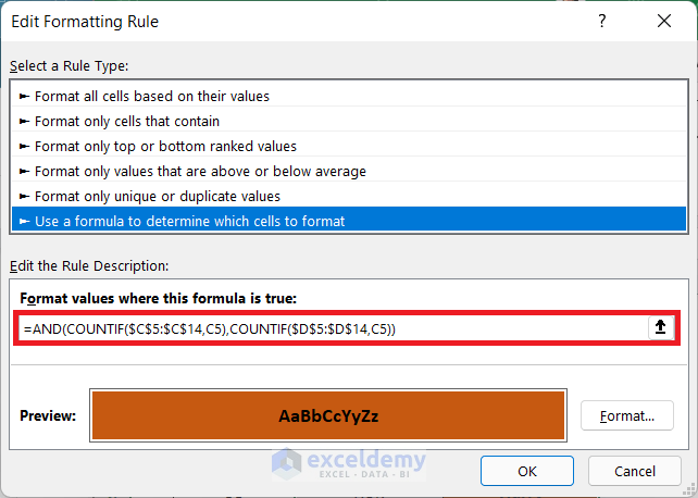
- Choose the Use a formula to determine which cells to format option.
- Copy the following formula into the empty box below Format values where this formula is true.
=AND(COUNTIF($C$5:$C$14,C5),COUNTIF($D$5:$D$14,C5))
- Select the Format option. Choose your formatting.
- In the Fill tab, select the cell fill color.
- Click OK to close the Format Cells dialog box.
- Click OK to close the New Formatting Rule box.
- You will see the cells containing duplicate values in columns C and D got the chosen cell format.
Breakdown of the Formula
We are doing this breakdown for cells C5 and D6.
COUNTIF($C$5:$C$14,C5): This function returns 1.
COUNTIF($D$5:$D$14,C5): This function returns 1.
AND(COUNTIF($C$5:$C$14,C5),COUNTIF($D$5:$D$14,C5)): This formula returns True. If both is 1, that means it has found a match.
Read More: How to Highlight Duplicates in Two Columns Using Excel Formula
Method 4 – Applying VBA Macro to Highlight Duplicates in Multiple Columns
Steps:
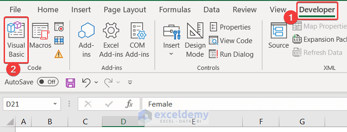
- Go to the Developer tab and click on Visual Basic. If you don’t have that, you have to enable the Developer tab. You can also press Alt + F11.
- A dialog box will appear.
- In the Insert tab, click Module.

- Copy the following visual code in the editor box.

Sub Highlight_Duplicate_in_Multiple_Column()
Dim rng_1 As Range, rng_2 As Range, cell_1 As Range, cell_2 As Range
Dim output As Range, output2 As Range
xTitleId = "Duplicate in Multiple Columns"

Set rng_1 = Application.Selection
Set rng_1 = Application.InputBox("Select Range1 :", xTitleId, rng_1.Address, Type:=8)
Set rng_2 = Application.InputBox("Select Range2:", xTitleId, Type:=8)

Application.ScreenUpdating = False

For Each cell_1 In rng_1
    Data = cell_1.Value
    For Each cell_2 In rng_2
        If Data = cell_2.Value Then
            cell_1.Interior.ColorIndex = 36
            cell_2.Interior.ColorIndex = 36
        End If
    Next
Next

Application.ScreenUpdating = True
End Sub- Close the Editor tab.
- From the View ribbon, click on Macros and go to View Macros.
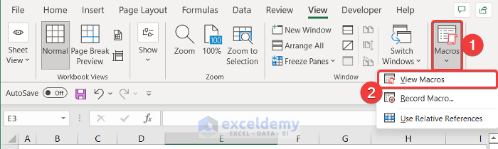
- A new dialog box called Macro will appear. Select Highlight_Duplicate_in_Multiple_Column.
- Click on the Run button to run this code.
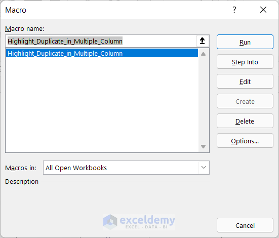
- Duplicated values will get highlighted.
Read More: How to Highlight Duplicates but Keep One in Excel
Download the Practice Workbook
Related Articles
- How to Highlight Duplicates in Excel with Different Colors
- How to Highlight Duplicate Rows in Excel
- Highlight Duplicates across Multiple Worksheets in Excel
- [Fix:] Highlight Duplicates in Excel Not Working
<< Go Back to Highlight Duplicates in Excel | Learn Excel
Get FREE Advanced Excel Exercises with Solutions!
