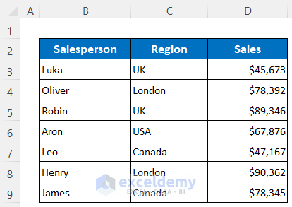
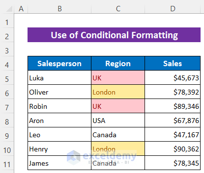
Below, we will go over two quick and useful methods to highlight duplicates in Excel. To explore the methods, we’ll use the following dataset, representing a salesperson’s sales in different regions.
Method 1 – Apply Conditional Formatting to Highlight Duplicates in Excel with Different Colors
Steps:
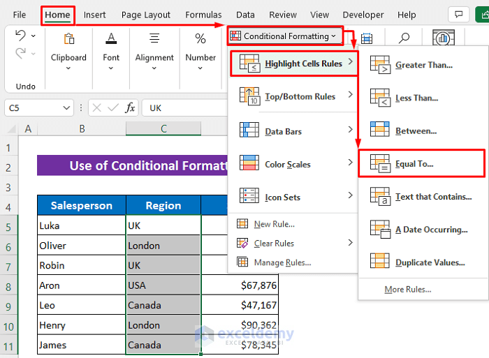
- Select the data range where you want to apply Conditional Formatting. I selected C5:C11.
- Click: Home > Conditional Formatting > Highlight Cells Rules > Equal To
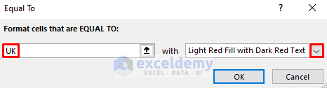
- A Conditional Formatting dialog box named Equal To will open
- Type the name of the Region for the duplicates you are looking for. I typed UK in the Format cells that are EQUAL TO:
- Click on the drop-down icon from the right side of the dialog box and select your desired color.
- Press OK.
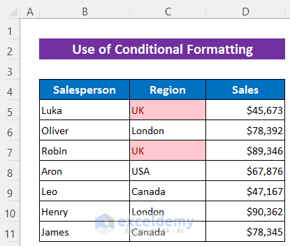
You will get all the duplicates for the region of the UK highlighted with your selected color.
Highlight the duplicates for another Region – London.
- Follow the first step to open the Conditional Formatting dialog box.
- Type the region name – London in the Format cells that are EQUAL TO:
- Select your desired color from the drop-down list.
- Press OK.

Duplicates of the London region are now highlighted with a different color.
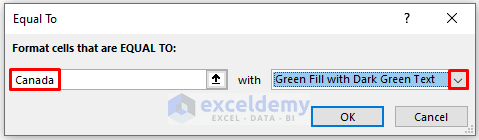
- To highlight the duplicates for the Canada region, follow the first step to open the Conditional Formatting dialog box.
- Write Canada in the Format cells that are EQUAL TO: box and select another color from the drop-down list.
- Press OK.
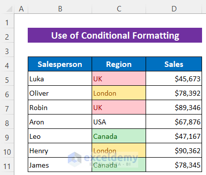
All different duplicate Regions are highlighted with different colors.
Read More: How to Highlight Duplicates in Multiple Columns in Excel
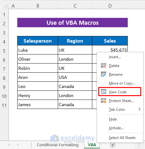
Method 2 – Embed Excel VBA to Highlight Duplicates with Different Colors
Using VBA macros is quicker than the first method.
Steps:
- Right-click on the sheet title to open the VBA window.
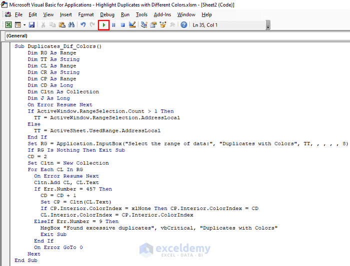
- Copy the following codes to the VBA window.
Sub Duplicates_Dif_Colors()
    Dim RG As Range
    Dim TT As String
    Dim CL As Range
    Dim CR As String
    Dim CP As Range
    Dim CD As Long
    Dim Cltn As Collection
    Dim J As Long
    On Error Resume Next
    If ActiveWindow.RangeSelection.Count > 1 Then
      TT = ActiveWindow.RangeSelection.AddressLocal
    Else
      TT = ActiveSheet.UsedRange.AddressLocal
    End If
    Set RG = Application.InputBox("Select the range of data:", "Duplicates with Colors", TT, , , , , 8)
    If RG Is Nothing Then Exit Sub
    CD = 2
    Set Cltn = New Collection
    For Each CL In RG
      On Error Resume Next
      Cltn.Add CL, CL.Text
      If Err.Number = 457 Then
        CD = CD + 1
        Set CP = Cltn(CL.Text)
        If CP.Interior.ColorIndex = xlNone Then CP.Interior.ColorIndex = CD
        CL.Interior.ColorIndex = CP.Interior.ColorIndex
      ElseIf Err.Number = 9 Then
        MsgBox "Found excessive duplicates", vbCritical, "Duplicates with Colors"
        Exit Sub
      End If
      On Error GoTo 0
    Next
End Sub- Click on the Run icon to run the codes.
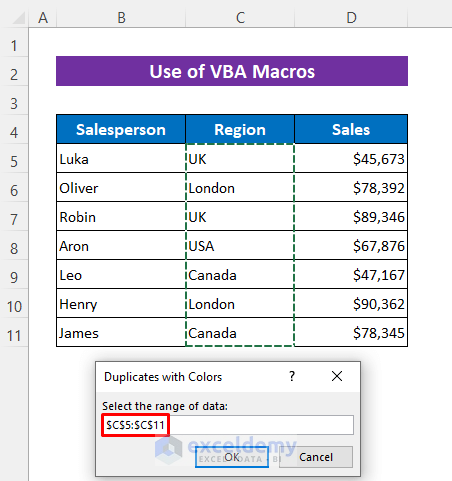
An lnputBox will pop up to select the data range.
- Select the data range C5:C11 by dragging it with your mouse.
- Press OK.
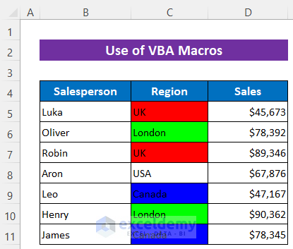
Excel has highlighted all the duplicates with different fill colors.
Read More: [Fix:] Highlight Duplicates in Excel Not Working
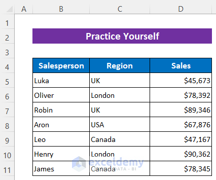
Practice Section
You will get a practice section in the Excel file given above to practice the explained methods.
Download Practice Workbook
You can download the free Excel template from here and practice on your own.
Related Articles
- How to Highlight Duplicates but Keep One in Excel
- Highlight Cells If There Are More Than 3 Duplicates in Excel
- How to Highlight Duplicates in Two Columns in Excel
- How to Highlight Duplicates in Two Columns Using Excel Formula
- How to Highlight Duplicate Rows in Excel
- Highlight Duplicates across Multiple Worksheets in Excel
<< Go Back to Highlight Duplicates in Excel | Learn Excel
Get FREE Advanced Excel Exercises with Solutions!

Hi, thanks for the instruction. I have applied the VBA for my worksheet. I have more than 100 duplicates and the macro does not cover all the duplicate values. How can I modify the code? Thanks a lot.
Hello, DANDELION!
Please select the range properly, this macro also works for more than 100 duplicates. There is no limitation. All you need to do is after running the code select the range properly.
Good Luck!
Regards,
Sabrina Ayon
Author, ExcelDemy.
I am working with six columns separated by other data, as follows A1 and A2 merged data related is on cells b2, and b3, then it repeats for C1 and C2 merged, data related on d2 and d3, and so on. It repeats six times to the left and then six times down. The duplicate values I need to check is on the merged cells, for each duplicate value that is different use another color, if there is no duplicate no color . Any advise?
Hi Maikel,
Can you share your Excel file with us, kindly? So that we may have a look at it and give you some suggestions.
Is there a way to modify the code so that you can choose the colors?? or choose a color pallette?
Hi Anna,
Thanks for commenting. There are 13 commands under the Interior application. When you put a dot (.) after the Interior application you will find the commands. there are Color, Colorindex, Pattern, ThemeColor, etc in the command section. But all the commands have the built-in color code that’s why you won’t be able to choose a specific color using this code. but while you working with blanks you can insert the RGB command and the Custom Color Code. In our case, it is not possible as we have to maintain the same color for the duplicates. Hope, you understand our answer.
Regards,
Fahim Shahriyar Dipto
Excel & VBA Content Developer.
Is there any way to change the color scheme? The ones in this are too dark.
Hi Carrie,
Greetings. Thanks for commenting. Yes, you can change the color scheme by following the below process.
Select the data range where you want to apply Conditional Formatting. Then click as follows: Home > Conditional Formatting > Highlight Cells Rules > Equal To.
Soon after, a Conditional Formatting dialog box named Equal To will open up
Type the name of the Region for what you are looking for duplicates.
Then click on the drop-down icon from the right side of the dialog box and select Custom Format.
Therefore, the Format Cells window will appear, and select the Fill option. Then choose your desired color.
Finally, just press OK
The code is only working for the first 109 rows out of a document that contains 6000 can you point me in the right direction to get this working fully?
Hi Keaton, thanks for your query. As the code has no limitation on the number of rows, it should work in your case. Maybe the code worked for the first 109 rows only because you only selected the first 109 rows in the prompt. Kindly select the entire dataset while running the code. Hopefully, it will do the job for you. If the code still doesn’t work, you can share your file using our Exceldemy forum(https://exceldemy.com/forum/).
the same is happening to me. I have 1000 lines in my spreadsheet with many different groups of duplicates. the code stops working around line 100 on my spreadsheet and enters an infinite loop. I’ve tried stepping into the debugging and it does go through all the correct lines in the code and it SHOUD be coloring the very next cell, but for some reason it’s not????. after stopping and restarting the program, selecting the next range (100-1000), it again colors the duplicates all the way up to around line 200 then stops again.
Hello Heather,
May be the problem is related to Excel’s limitations when applying multiple conditional formatting rules or when handling a large range with VBA. This could be causing the code to slow down or enter an infinite loop. A possible solution is to break the range into smaller sections or optimize the code by limiting the number of FormatConditions applied at once.
Here, I’m Reviewing the loop logic and error handling, could also help prevent the program from freezing.
I used FormatConditions.AddUniqueValues with xlDuplicate to highlight duplicates directly.
Then used the Chunk size logic is retained to process large ranges in smaller sections.
All the ranges are based on our existing Excel sheet.
Use the updated VBA code:
Regards
ExcelDemy
Hi there,
For the VBA code, cells with blank entries are also colour-coded. How may I modify the code to avoid this issue from happening?
Hi there, for the VBA code,
In my own workbook, cells with blank entries are also color-coded. Please advise on how i can modify the code so as to prevent cells with blank entries to be left with no color fill?
This code will solve your problem. The code has a condition checking values blank or not.
Output:
Thanks so much for the VBA. It was really helpful 🙂
Margaret (from the Philippines
Dear Margaret,
You are welcome.
Regards
ExcelDemy
Hi there,
Some of the background colors produced by the VBA are too dark for the font to be visible. Where in the code, do I add the option to make the font to use a lighter color on a darker background and vice-versa?
Regards
AML
Hello AML,
You can add IF statement to adjust font color based on background brightness in the VBA code. You can add a condition that sets the font color to white for darker backgrounds and black for lighter ones.
Condition to add lighter color on a darker background and vice-versa:
Place this inside the loop where you’re setting background colors. This will ensure visibility based on the background color.
Regards
ExcelDemy