The DGET function in Excel is a database function and is designed to return only one record. In case you have multiple matches and need to return multiple records in Excel, you cannot use the DGET function anymore. The DGET function returns #NUM! error in these cases. So, you have to use alternatives to DGET if you have to return multiple records that match certain criteria.
Download Practice Workbook
You can download the following practice book to practice while reading this article.
Can Excel DGET Function Return Multiple Records?
Here, we will answer this question using an example.
- In the following image, we are showing some product details of a shop. We have set 3 sets of criteria: product+size+color, product+size, and only product names. We are trying to get the price of these matches using the DGET function. But each time, we get a #NUM! error.
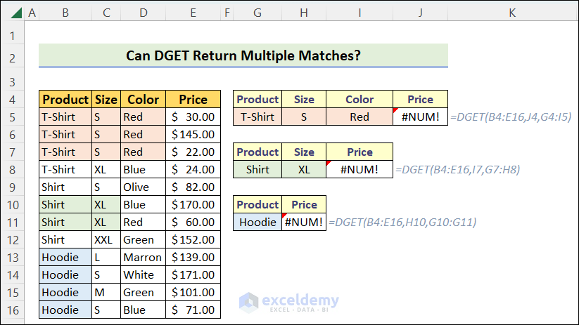
- For example, We see that the T-Shirt+S+Red criteria combination has 3 matches in the main data. But we are failing to return all these records using the DGET function.
- The same thing happens to the other sets of criteria and matches.
- So, as we have said already, the answer is- NO. DGET cannot return multiple records.
- Let’s see what support.microsoft.com says,
“If more than one record matches the criteria, DGET returns the #NUM! error value.”
Anyway, what will we do then? We will discuss this in the next section.
4 Alternatives to Excel DGET Function to Return Multiple Records
We have 4 suitable alternatives to DGET function when we are to return multiple records in Excel (Is there any more? Share your thoughts in the comment box!).
1. Using FILTER Function to Return Multiple Records
The first (and the best we have got) way is using the FILTER function of Excel. How to use this function in this case?
Note:
The FILTER function is only available in Excel 2019 or later versions. If you are a user of Excel 2016 or earlier versions, see the 3rd method of this article.
Case-i: Three Criteria Combination
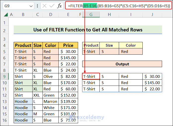
- To return all the prices that match the 3 criteria combination (Product=T-Shirt, Size=S, Color=Red), use the following formula in cell J5.
=FILTER(E5:E16,(B5:B16=G5)*(C5:C16=H5)*(D5:D16=I5))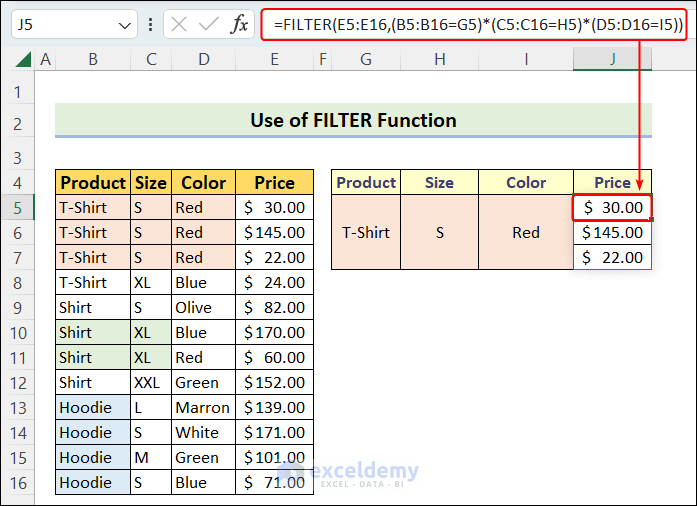
- Here, E5:E15=Price column (the column from which you want to return records)
- B5:B16=Product column (the column in which you will test the 1st criteria)
- C5:C16=Size column (column of 2nd criteria match)
- D5:D16=Column of 3rd criteria match, Color column
- (B5:B16=G5)*(C5:C16=H5)*(D5:D16=I5) generates a AND type criteria and FILTER function returns all the matching prices from E5:E16. If this combined criteria matches the 5th row, the price from E5 will be returned, and so on.
Case-ii: Two Criteria Combination
- For two-criteria combination, use the following formula.
=FILTER(E5:E16,(B5:B16=G10)*(C5:C16=H10))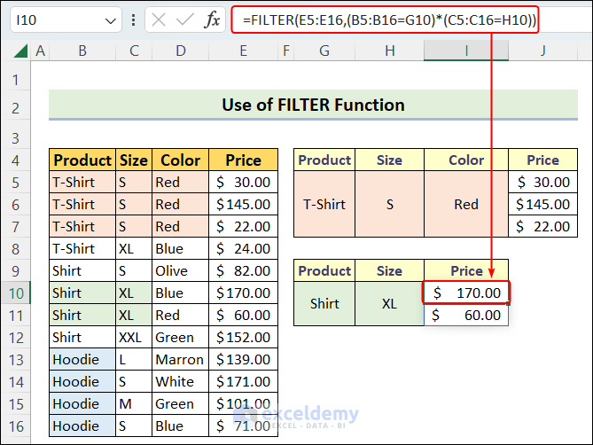
Case-iii: Single Criterion
- For a single criterion, the following formula will go.
=FILTER(E5:E16,B5:B16=G14)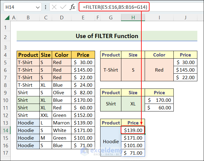
To return all the entire rows that match any criteria, just change the Array argument of the FILTER function from E5:E16 (only a single column) to B5:E16 (the entire dataset).
Read More: How to Use Database Functions in Excel (With Examples)
2. Using a Combination of TEXTJOIN and IF Functions
In this formula, the TEXTJOIN function will return all the records in a single cell. We will also insert the IF function in this formula to check the criteria.
- In this example, let’s assume that the criterion is only the product name (single criterion): Hoodie. We want to know all the Hoodie prices in a single cell.
- Now, write the following formula in cell H5 and press Enter.
="$"&TEXTJOIN(" , $",TRUE,IF(B5:B16=G5,E5:E16,""))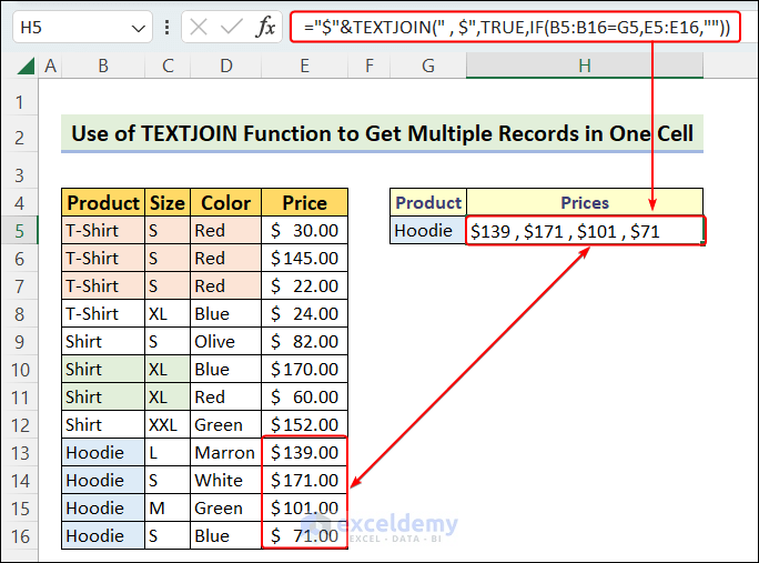
- If you don’t need to have these outputs in USD format, then the formula will be simpler.
=TEXTJOIN(" , ",TRUE,IF(B5:B16=G5,E5:E16,""))- To match two criteria and return records, use the following formula instead:
="$"&TEXTJOIN(" , $",TRUE,IF((B5:B16=G5)*(C5:C16=H5),E5:E16,""))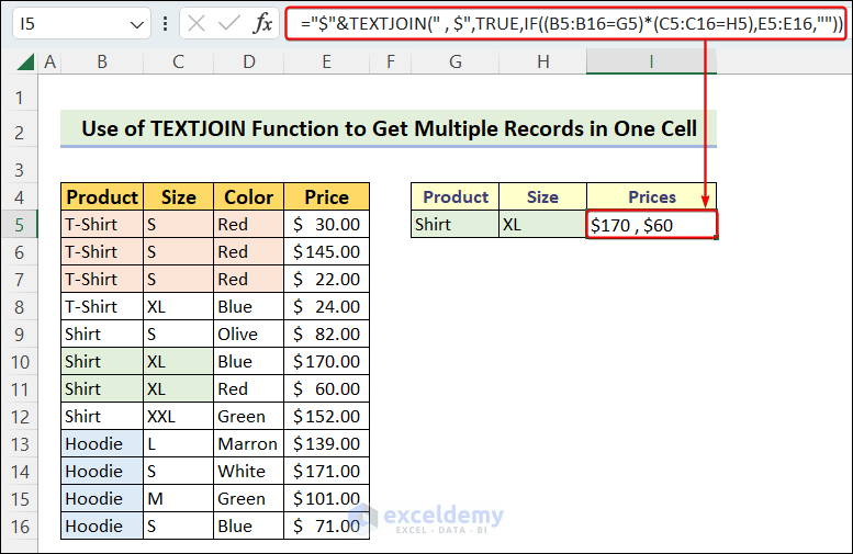
Or,
=TEXTJOIN(" ,",TRUE,IF((B5:B16=G5)*(C5:C16=H5),E5:E16,""))- To return three criteria, the formula will be as follows,
="$"&TEXTJOIN(" , $",TRUE,IF((B5:B16=G5)*(C5:C16=H5)*(D5:D16=I5),E5:E16,""))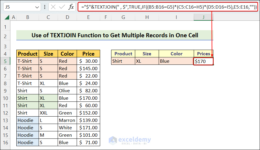
Or,
=TEXTJOIN(" ,",TRUE,IF((B5:B16=G5)*(C5:C16=H5)*(D5:D16=I5),E5:E16,""))Read More: How to Use DCOUNT Function in Excel (5 Suitable Examples)
3. Using a Combination of INDEX, IF, SMALL and ROW Functions
There is another formula you can use to return multiple records. It uses the combination of INDEX, IF, SMALL, and ROW functions. This formula is a substitute for the FILTER formula mentioned here if you don’t use Excel 2019 or later versions.
- To apply this formula for a single criterion, write the following in cell H5 and hit the Enter button.
=IFERROR(INDEX($E$5:$E$16,SMALL(IF($G$5=$B$5:$B$16,ROW($B$5:$B$16)-ROW($B$5)+1), ROW(1:1))),"" )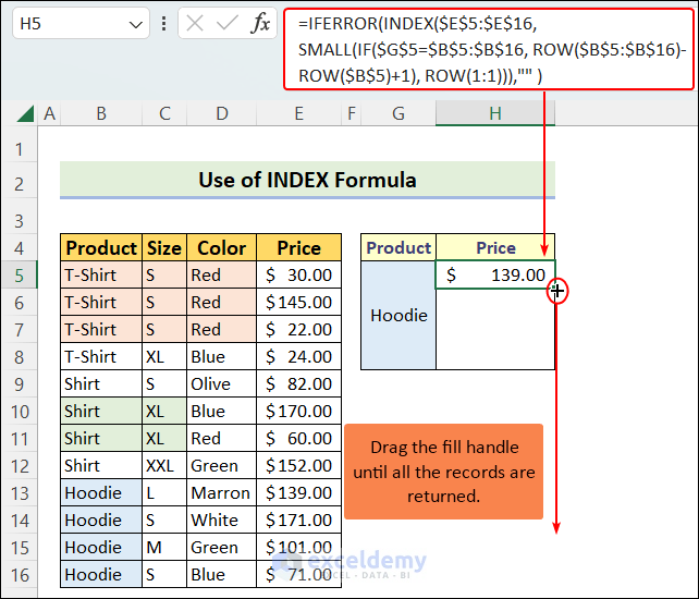
- This formula is not an array formula, so you have to drag the fill handle down to get the next records. Drag it until you reach a blank cell.
- The IFERROR function is inserted here to return an empty string when there is no match while dragging it down.
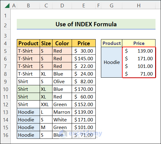
- After all these, you will get all the records just like the image below.
Formula Breakdown:
Full Formula: =IFERROR(INDEX($E$5:$E$16,SMALL(IF($G$5=$B$5:$B$16, ROW($B$5:$B$16)-ROW($B$5)+1), ROW(1:1))),”” )
- ROW($B$5:$B$16)-ROW($B$5)+1
This ROW formula returns all the serial numbers of the products, starting from 1. ROW($B$5:$B$16) returns {5;6;7;8;9;10;11;12;13;14;15;16} which is the array of actual row numbers of the Products. When we minus ROW($B$5) or {5} from this array, the array becomes {0;1;2;3;4;5;6;7;8;9;10;11}. Now adding 1 will make this array as {1;2;3;4;5;6;7;8;9;10;11;12}, which includes the serial number of all the products.
- IF($G$5=$B$5:$B$16, ROW($B$5:$B$16)-ROW($B$5)+1)
Here, the IF function checks criteria $G$5=$B$5:$B$16. If it is true, then the IF function returns the serial number in {1;2;3;4;5;6;7;8;9;10;11;12} array (output of ROW($B$5:$B$16)-ROW($B$5)+1). If false, the function returns FALSE. Since this criteria is true only for B13:B16, the IF function returns FALSE for the rest of the products. So, the output is: {FALSE;FALSE;FALSE;FALSE;FALSE;FALSE;FALSE;FALSE;9;10;11;12}.
- SMALL(IF($G$5=$B$5:$B$16, ROW($B$5:$B$16)-ROW($B$5)+1), ROW(1:1))
Here comes the SMALL function on the scene. Let’s write this part in simpler form first: SMALL({FALSE;FALSE;FALSE;FALSE;FALSE;FALSE;FALSE;FALSE;9;10;11;12}, ROW(1:1)). Here, the ROW(1:1) part returns 1 and hence the SMALL function returns the smallest number in the {FALSE;FALSE;FALSE;FALSE;FALSE;FALSE;FALSE;FALSE;9;10;11;12} array. And it’s 9.
- INDEX($E$5:$E$16,SMALL(IF($G$5=$B$5:$B$16, ROW($B$5:$B$16)-ROW($B$5)+1), ROW(1:1)))
Finally this formula becomes INDEX($E$5:$E$16,{9}). So, the INDEX function will return the 9th item of the $E$5:$E$16 array. $E$5:$E$16 means {30;145;22;24;82;170;60;152;139;171;101;71}. And its 9th item is 139. And this is the final output.
- When you drag down this formula, the records that match the set criteria will appear one after another down the column. When all of them are there and you still drag the formula down, you will see #NUM! error. The IFERROR function here makes sure that, when this situation occurs, you will have empty strings instead, and you can have a clear spreadsheet without deleting anything.

- To apply the formula for two criteria, use the following formula. Modify the formula according to your case, or leave us a comment if you fail to do so.
=IFERROR(INDEX($E$5:$E$16, SMALL(IF(COUNTIF($G$5, $B$5:$B$16)*COUNTIF($H$5, $C$5:$C$16), ROW($B$5:$B$16)-MIN(ROW($B$5:$B$16))+1), ROW(A1)), COLUMN(A1)),"")
- For 3 criteria matches, the formula will be as follows.
=IFERROR(INDEX($E$5:$E$16, SMALL(IF(COUNTIF($G$11, $B$5:$B$16)*COUNTIF($H$11, $C$5:$C$16)*COUNTIF($I$11, $D$5:$D$16), ROW($B$5:$B$16)-MIN(ROW($B$5:$B$16))+1), ROW(A1)), COLUMN(A1)),"")Read More: How to Use DOLLAR Function in Excel (5 Suitable Examples)
4. Using Advanced Filter to Return Multiple Records
Excel has a fantastic feature called the Advanced Filter which you can use to return multiple records for certain matches. Let’s see how to use this in our case.
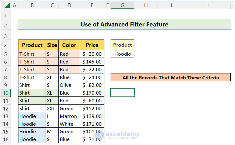
- The following image shows the source dataset and criteria set.
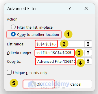
- Now, go to the Data tab and select the Advanced command from the Sort & Filter group.

- In the following window, select the option “Copy to another location”.
- Then select the List range. This is the source range from which you want to extract multiple matched records. In our case, it’s B4:E16.
- After that, select the Criteria range, which is G4:G5 in our case.
- Then choose a suitable starting location to copy the filtered records.
Select the List range and Criteria including the Column Labels, otherwise, you will get a faulty result.
- After pressing OK, you will have this!

Note:
You can also apply multiple criteria with the Advanced Filter feature.
Read More: How to Use Excel DSUM Function (4 Appropriate Examples)
Conclusion
So, try one of these methods if you fail to use the DGET function to return multiple records in Excel. Were these helpful? Please leave us your feedback in the comment box.
Related Articles
- How to Determine If a Number Is Even in Excel (4 Suitable Ways)
- Use DSUM Function with Multiple Criteria in Excel
- How to Use Excel DGET with Dynamic Criteria
- How to Use EDATE Formula for Days (3 Ideal Examples)
<< Go Back to Excel DGET Function | Excel Functions | Learn Excel

