Have you ever wondered how to apply the DGET function of Excel for multiple dynamic criteria? The DGET function of Microsoft Excel is one of the database functions it has. It extracts a single record from a database that matches one or more criteria we specify. So, to apply dynamic criteria, there is no complicacy with the DGET function, the only additional thing we have to do is create a dynamic criteria list. In this article, we will see how to do this with detailed steps and proper illustrations.
Download Practice Workbook
You can download the following practice workbook for your practice while reading this article.
Steps to Apply DGET Function with Dynamic Criteria in Excel
1st Step: Collect Sample Data to Create a Database for DGET Function
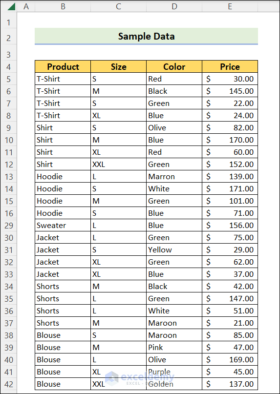
- To start with, we will first create a database with our data.
- In the following image, we have some product data with their sizes, colors, and prices.
2nd Step: Add Field and Criteria for DGET Function
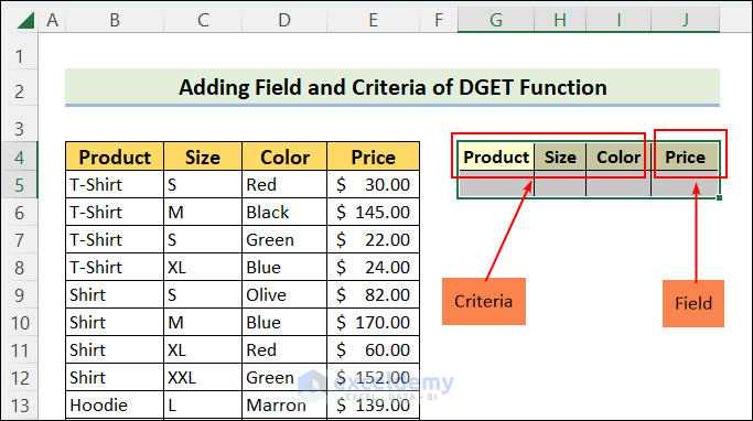
- The next step is to add fields and criteria to search for, with the DGET function.
- Here, we have just copied the B4:E4 cells and pasted them into cells G4:J4.
- G4:I4 are the criteria and J4 is the field.
Note:
- Field: Field is the 2nd argument of the DGET function. It is the name or index to count for which you are searching.
- Criteria: It is the 3rd argument of the DGET function. It is the criteria that apply to the DGET function, including the headers.
3rd Step: Add a Helper Column That Will Have an Updated Unique List of Products
- Before creating a dynamic dropdown list for criteria, we will need to add some helper columns.
- In these columns, we will create a unique list of Products, Sizes, and Colors.
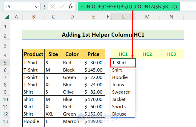
- Here, we have added 3 helper columns for 3 criteria: HC1, HC2, and HC3 (columns L, M & N).
- Write the following formula in cell L5 to get a unique list of the products from the source list.
=UNIQUE(OFFSET(B5,0,0,COUNTA($B:$B)-2))
- As a result, you will have a unique list of criteria.
Note:
This is an array formula. If you are not an Office 365 user, then you may need to press Ctrl+Shift+Enter to apply an array formula.
Formula Explanation:
Since you are searching for a way to apply dynamic criteria with the DGET function, we have designed the formula in such a way that the helper column HC1 will always have a unique list of the Products.
I mean, if you add more items to the source data, the helper column will automatically update in accordance with the change.
Now, how does this formula work to make it possible?
Let’s dig deep.
- COUNTA($B:$B)-2
Output: 10
Explanation: In this piece of the formula, the COUNTA function counts the number of cells in column B that are not empty. Since there are two non-empty cells (B2 and B4) that are not of our consideration, so we minus 2 from COUNTA($B:$B) to count only the valid entries in the source data.
- OFFSET(B5,0,0,COUNTA($B:$B)-2)
Output: {“T-Shirt”;”Shirt”;”Shirt”;”Pant”;”Hoodie”;”Jeans”;”Sweater”;”Jacket”;”Shorts”;”Blouse”}
Explanation: Here, the OFFSET function starts from B5 (first data in the Product column) and remains in the same cell (denoted by 0 and 0, every 0 means the number of rows and columns at which number the function goes forward). So, OFFSET(B5,0,0,COUNTA($B:$B)-2)=OFFSET(B5,0,0,10) returns all the 10 valid items of column B).
- UNIQUE(OFFSET(B5,0,0,COUNTA($B:$B)-2))
Output: {“T-Shirt”;”Shirt”;”Pant”;”Hoodie”;”Jeans”;”Sweater”;”Jacket”;”Shorts”;”Blouse”}
Explanation: The UNIQUE formula now becomes- UNIQUE({“T-Shirt”;”Shirt”;”Shirt”;”Pant”;”Hoodie”;”Jeans”;”Sweater”;”Jacket”;”Shorts”;”Blouse”}). So it returns the unique items in this array, e.g. it counts Shirt only once, though this item occurs twice in the source data.
- Is this list dynamic? Test it by yourself by adding more items. The list will be automatically updated.
4th Step: Create 1st Dropdown List of Unique Items (Products List)
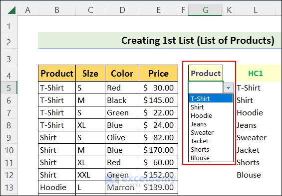
- Now, we are prepared to create the 1st dropdown list of product criteria.
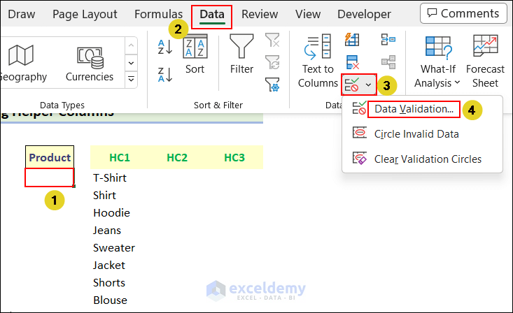
- To do this, first select cell G5 and go to the Data tab.
- From the Data Tools group, click on the Data Validation command.
- The following window will appear.
- From the Settings section, select List in the Allow: box and input the following formula in the Source: box.
=INDIRECT("$L$5#")
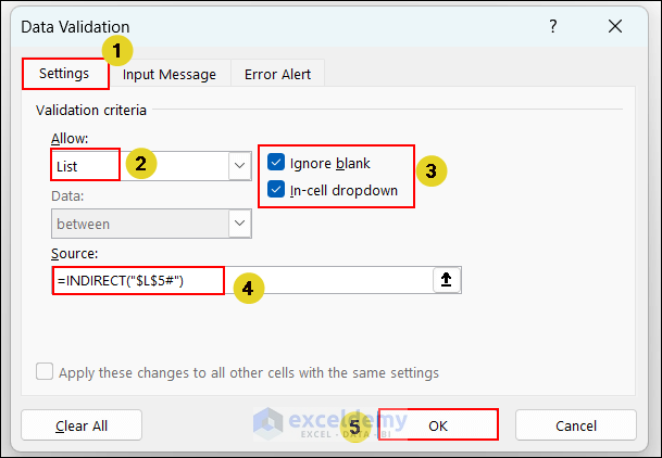
The INDIRECT function returns the value of $L$5# range. the # sign denotes the continuation of the range after L5 till there is data down the column. # is used for spilled range in Excel.
- Press OK.
- You will see the following drop-down list appear in your Excel spreadsheet.
5th Step: Add Next Helper Column That Will Have All Available Sizes for the Item Selected from 1st Dropdown List
- Now, we will create another helper column HC2, that will have the unique sizes for the product specified in cell G5.
- Enter the following formula in cell M5 to do this.
=IF(UNIQUE(FILTER(C:C,B:B=G5))=0,"Select a product in cell G5",UNIQUE(FILTER(C:C,B:B=G5)))Explanation:
- Here the FILTER function will search for entries in column C (size column) where B:B=G5 criteria match. And the UNIQUE function will then pick all the unique available sizes.
- If there is no match from FILTER function, then the UNIQUE function returns 0.
- To handle this, we have inserted the IF function, which will return a prespecified text (here, it is: “Select a product in cell G5”).
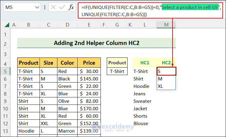
- When you select nothing in cell G5, the formula will tell you to do so.

6th Step: Create 2nd Dynamic Dropdown List (Unique List of Available Size, Dependent on the 1st List)
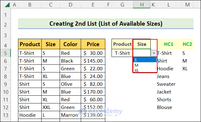
- Following the same way as in the 4th step, create a dropdown list for the available sizes in cell H5.
- This time, the formula to use the source data box is as follows:
=INDIRECT("$M$5#")
7th Step: Create the Last Dynamic Helper Column for Colors
- Use the following formula in cell N5 to create a helper column that has the dynamic list of colors for a certain set of products and sizes.
=IFERROR(UNIQUE(FILTER(D:D,(B:B=G5)*(C:C=H5))),"Select a size")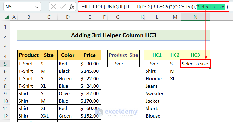
Explanation:
- This formula is similar to the formula in the 5th step.
- Here are some additional attributes in this formula. The IFERROR function is inserted here to tell you to select a size from the 2nd dropdown list if you haven’t selected any.
- The asterisk symbol in (B:B=G5)*(C:C=H5) combines the two logics B:B=G5 and C:C=H5 and creates a AND type criteria.
8th Step: Create the Last Dynamic Dropdown List (List of Colors for a Certain Product-Size Combination)
- Follow the same process we have applied in the 4th step to create this dropdown list of colors for a certain set of products and sizes in cell I5.
- This time, use the following formula to extract source data.
=INDIRECT("$N$5#")

Last Step: Finally Apply DGET with Dynamic Criteria in Excel
- Now, we are all set, write the following formula in cell J5:
=IFERROR(DGET(B4:E42,J4,G4:I5),"All criteria not set!")
The DGET function has the following syntax.
=DGET(database,field,criteria)
Hence,
- B4:E14= Database
- J4= Field
- G4:I5= Criteria with headers
- Since we haven’t selected any criteria, the formula is telling us, “All criteria not set!”.
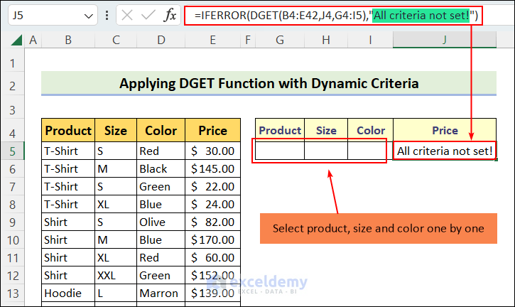
- Now, if we specify criteria one by one, we will see the output in cell J5, generated by the DGET function!
Quick Notes
- Product, Size, Color & Price are the header names of the source data. Note that, these names must be kept the same in the copied section (G4:J4).
- If you make even a small change in the header names, the DGET will not work properly.
- You can assign a number for the Field argument in the DGET formula. In this article, you could write 4 instead of J4 as the field in =DGET(B4:E14,J4,G4:I5) formula.
- But you must keep the criteria labels the same as the source data.
Things to Remember
- The DGET function cannot return records for multiple matches. In such a case, the DGET function returns #NUM! error.
If we see the following screenshot, we will agree that the DGET function does not work for multiple records. One of the best alternatives to this problem is using the Advanced Filter command of Excel.

Here I am showing how to use this feature for multiple records.
- Go to the Data tab and find the Sort & Filter group.
- After that, click on the Advanced button.

- The Advanced Filter pop-up will appear. Here you have some range or location to choose from.
- First, select the Copy to another location option.
- Then select the List range. It’s the whole database: B4:F42.
- Then select the Criteria range: H4:J5.
- After that, select a suitable starting location, where you want to place the multiple records.
- Mark the “Unique records only” box.

- All are set. Now, press OK.
- Look at the following image. All the records that match the criteria are present here now.

- The DGET function returns #VALUE! error in case of no match.
- In this article, we have designed the whole model in such a way that, hopefully, you will never face an erroneous case. If you face any, leave us a comment.
Concluding Words
So, here we are at the end of our discussion. I hope this write-up will help you in learning how to apply the DGET function of Excel with dynamic criteria. If you have further queries regarding this topic, let us know in the comment box. Also, don’t forget to visit our blog ExcelDemy for more Excel-related articles. Happy Excelling!
<< Go Back to Excel DGET Function | Excel Functions | Learn Excel
Get FREE Advanced Excel Exercises with Solutions!
