If you are looking for some special tricks to know how to use the DOLLAR function in Excel, you’ve come to the right place. We’ll show 5 suitable examples to use the DOLLAR function in Excel. This article will discuss every step of the examples. Let’s follow the complete guide to learn all of this.
DOLLAR Function: Summary & Arguments
- Summary:
DOLLAR function is a TEXT function for converting numbers to text using currency format with decimal points rounded to the specified number. There is no set currency symbol for the Dollar. It depends on your local language settings whether it uses ($#,##0.00_);($#,##0.00) number format.
- Syntax:
The syntax of the Dollar function is as follows:
=DOLLAR(number, [decimals])

- Arguments:
| Argument | Required/Optional | Explanation |
|---|---|---|
| number | Required | References to cells that contain numbers, and formulas that evaluate into numbers. |
| [Decimals] | Optional | After the decimal point, the number of digits is listed. In the case of a negative number, the decimal point is rounded to the left. The decimal point is assumed to be two if you want to omit the decimal point. |
- Return Value:
This application converts a number into text in the form of a currency.
- Available in Version:
Office 365 ■ Excel 2019 ■ Excel 2016 ■ Excel 2013 ■ Excel 2011 for Mac ■ Excel 2010 ■
Excel 2007 ■ Excel 2003 ■ Excel XP ■ Excel 2000.
The following section demonstrates the use of the DOLLAR function in Excel using five practical and tricky examples. The following dataset contains two columns that we will use for demonstration purposes. The number column contains the number, and the Result column contains the result of the converted text.

You should learn and apply these to improve your thinking capability and Excel knowledge. We use the Microsoft Office 365 version here, but you can utilize any other version according to your preference.
1. Converting Number into Text
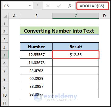
In the first illustration, we’ll show how to use the DOLLAR function to convert a number into text. In this case, we won’t enter any numbers in the argument. The function will therefore convert a number into text with a two-digit decimal point. Let’s walk through the following steps to do the task.
📌 Steps:
- First, write down the following formula in cell D5.
=DOLLAR(B5)
- Then, press Enter.
- Therefore, you will get the following output.
- Next, drag the Fill Handle icon to fill the other cells with the formula.
- Consequently, you will be able to convert numbers into text with two-digit decimal points.

2. Getting Number in Text with Decimal Points Format
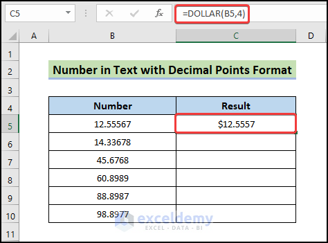
Here, we’ll show you how to use the DOLLAR function to get numbers in text with decimal point formatting. To accomplish this, we must enter a number in the DOLLAR function’s argument option.
📌 Steps:
- First, write down the following formula in cell D5.
=DOLLAR(B5,4)
Here, we enter 4 in the DOLLAR function’s argument to get a text with the four-digit decimal point.
- Then, press Enter.
- Therefore, you will get the following output.
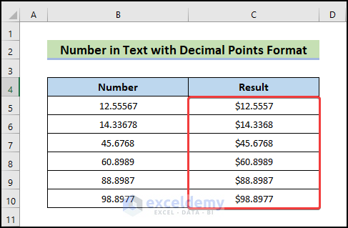
- Afterward, drag the Fill Handle icon to fill the other cells with the formula.
- Consequently, you will be able to get a text with a four-digit decimal point.
3. Transforming Number to Text Without Decimal Point
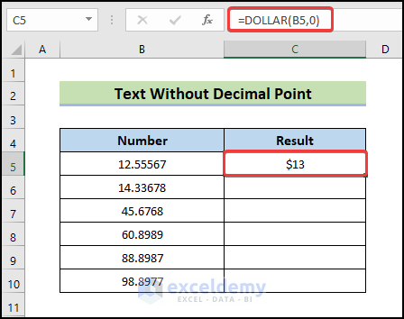
In this method, we will show how to transform numbers into text without a decimal point. In order to do so, we have to enter zero into the argument option of the DOLLAR function. Let’s follow the following steps to do the task.
📌 Steps:
- First, write down the following formula in cell D5.
=DOLLAR(B5,0)
- Then, press Enter.
- Therefore, you will get the following output.
- Next, drag the Fill Handle icon to fill the other cells with the formula.
- Consequently, you will be able to transform numbers into text without a decimal point.

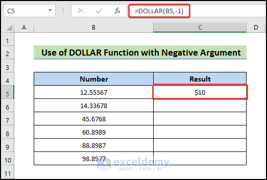
4. Using the DOLLAR Function with a Negative Argument
Now, we will show how to use the DOLLAR function with a negative argument. If we specify a negative argument, numbers will be rounded to the left of the decimal point. In order to do so, we have to enter negative numbers into the argument option of the DOLLAR function. Let’s follow the below steps.
📌 Steps:
- First, write down the following formula in cell D5.
=DOLLAR(B5,-1)
- Then, press Enter.
- Therefore, you will get the following output.
- Next, drag the Fill Handle icon to fill the other cells with the formula.
- Consequently, you will be able to transform numbers into text with a negative argument.

5. Joining Text with Excel DOLLAR Function
In this last example, we will demonstrate how to join text with the Excel DOLLAR function. Follow the following process.
📌 Steps:
- First, write down the following formula in cell D5.
="Total Amount " & DOLLAR(B5)
- Then, press Enter.
- Therefore, you will get the following output.

- Next, drag the Fill Handle icon to fill the other cells with the formula.
- Consequently, you will be able to join text with the currency format of the number as shown below.

💬 Things to Remember
✎ A non-numeric argument will result in a #VALUE! error.
✎ After converting a number with the Excel Dollar function, it is saved in Excel as text. As a result, it can’t be employed in numerical computations.
Download Practice Workbook
Download this practice workbook to exercise while you are reading this article. It contains all the datasets in different spreadsheets for a clear understanding. Try it yourself while you go through the whole process.
Conclusion
That’s the end of today’s session. I strongly believe that from now on you may know how to use the DOLLAR function in Excel. If you have any queries or recommendations, please share them in the comments section below. Don’t forget to check our website Exceldemy.com for various Excel-related problems and solutions. Keep learning new methods and keep growing!
<< Go Back to Excel Functions | Learn Excel
Get FREE Advanced Excel Exercises with Solutions!
