We are used to applying the COUNTIF function in Excel to count the cells according to given criteria but it’s a little bit difficult to count the cells that don’t contain multiple criteria. In this article, we will learn about how to count cells that are not equal to many things using the COUNTIF function in Excel.
Here is an overview of this article.
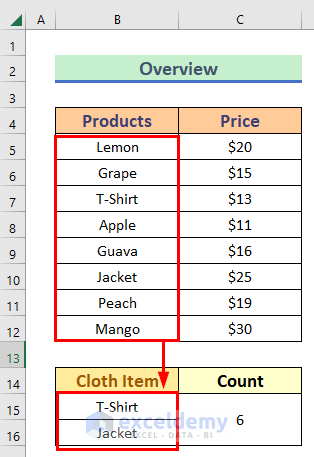
Use of COUNTIF Function That Does Not Contain Multiple Criteria in Excel
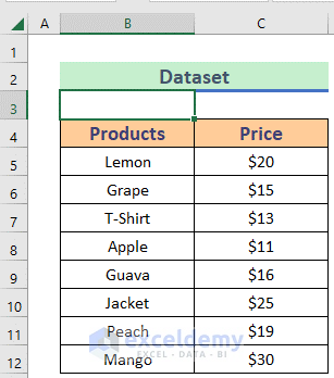
Let’s get introduced to our dataset first. I have placed some fruit and cloth items and their prices in the dataset.
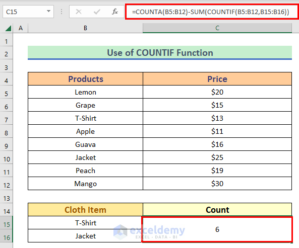
Now I’ll use the COUNTIF function, SUM function, and COUNTA function to exclude the cloth items from the fruit items. The SUM function adds values. And the COUNTA function will calculate the number of cells that are not blank within a given set of values. I have merged Cells C15 and C16 to apply the formula.
Steps:
➥ Activate the merged cell and write the formula given below-
=COUNTA(B5:B12)-SUM(COUNTIF(B5:B12,B15:B16))
➥ Just hit the Enter button to get the result.
Formula Breakdown
- COUNTIF(B5:B12,B15:B16) → It will count the cells from the range (B5:B12) according to the match criteria from the range (B15:B16)
- Output: {1;1}
- SUM(COUNTIF(B5:B12,B15:B16)) → Now the SUM function will sum up the array and will result in as
- Output: {2}
- COUNTA(B5:B12)-SUM(COUNTIF(B5:B12,B15:B16)) → The COUNTA function will count the total non-blank cells from the range (B5:B12). Then we subtracted the previous sum value from it. Then we’ll get our final result:
- Output: {6}
Read more: COUNTIF Multiple Ranges Same Criteria in Excel
Alternative to the Excel COUNTIF Function That Does Not Incorporate Several Criteria
Now I’ll show two alternative methods to count cells that are not equal to many things.
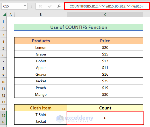
1. Use of COUNTIFS Function That Does Not Enclose Multiple Criteria in Excel
Here, we’ll use the COUNTIFS function to count cells that do not contain multiple criteria. COUNTIFS function is used to count the number of cells that fulfill a single criterion or multiple criteria in the same or different ranges in Excel.
Steps:
➥ By activating the merged cell type the formula-
=COUNTIFS(B5:B12,"<>"&B15,B5:B12,"<>"&B16)
➥ Then press the Enter button.
Formula Explanation
- B5:B12 → This is the criteria range.
- “<>”&B15 → This is the first criteria.
- “<>”&B16 → This is the second criteria.
- COUNTIFS(B5:B12,”<>”&B15,B5:B12,”<>”&B16) → This will return the output.
Read More: How to Apply COUNTIF Not Equal to Text or Blank in Excel
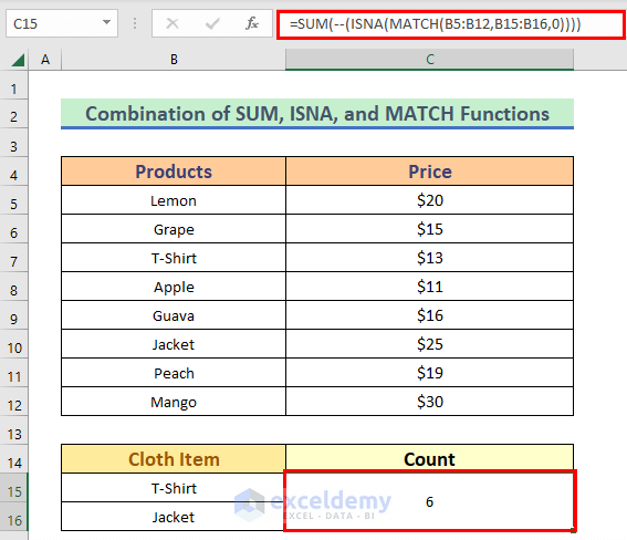
2. Combination of SUM, ISNA, and MATCH Functions That Does Not Contain Different Conditions in Excel
In this alternative method, we’ll use the combination of the SUM, ISNA, and MATCH Functions to do the same operation. The ISNA function checks whether a cell contains a “#N/A” error or not. The MATCH function searches for a value in an array and returns the relative position of that item.
Steps:
➥ In the merged cell write the formula given below-
=SUM(--(ISNA(MATCH(B5:B12,B15:B16,0))))
➥ Hit the Enter button to get the output.
Formula Breakdown
- MATCH(B5:B12,B15:B16,0) → The MATCH function is used to find cells not equal to “T-Shirt” or “Jacket“. This function returns the position of matching number values. It returns #N/A for all the other values.So it will return as-
- Output: {#N/A;#N/A;1;#N/A;#N/A;2;#N/A;#N/A}
- ISNA(MATCH(B5:B12,B15:B16,0)) → The #N/A results are the ones we’re looking for since they represent values not equal to “T-Shirt” or “Jacket“. Then we have used the ISNA function to convert these values to TRUE, and the numbers to FALSE. After that, the result will be as like-
- Output: {TRUE;TRUE;FALSE;TRUE;TRUE;FALSE;TRUE;TRUE}
- –(ISNA(MATCH(B5:B12,B15:B16,0))) → Then we have used a double negative to switch TRUE to 1 and FALSE to zero. The resulting array will look like this::
- Output: {1;1;0;1;1;0;1;1}
- SUM(–(ISNA(MATCH(B5:B12,B15:B16,0)))) → Finally, the SUM function will sum up the array and will give the counted result:
- Output:{6}
Read More: INDEX, MATCH and COUNTIF Functions with Multiple Criteria
Download Practice Workbook
You can download the free Excel template from here and practice on your own.
Conclusion
I hope all of the methods described above will be useful enough to count cells that do not contain multiple criteria. Feel free to ask any questions in the comment section and please give me feedback.
Related Articles
- Use COUNTIF with Wildcard in Excel
- Excel COUNTIFS Not Working
- COUNTIF vs COUNTIFS in Excel
- Excel COUNTIF for Multiple Criteria with Different Column
- COUNTIF Between Two Values with Multiple Criteria in Excel
- How to Use COUNTIF Function Across Multiple Sheets in Excel

