This article deals with the excel area chart data label position. An area chart is used to plot data arranged in rows or columns on a worksheet. You can use it to draw attention to the change over time and show the total value across a trend.
What Is Area Chart?
An area chart is used to plot data arranged in rows or columns on a worksheet. You can use it to draw attention to the change over time and show the total value across a trend. Excel allows us to insert both 2-D and 3-D area charts. There are three types of area charts available in excel. An area chart displays the change of values over time. A Stacked Area Chart shows the change in the contribution of each value over time. The 100% Stacked Area Chart shows the change in the contribution of each value over time in percentages.
How to Insert Excel Area Chart Data Label and Change Their Position
In this part, we will create an area chart to show the data labels and change their positions in area charts in Excel.
📌 Step 1: Organize Data
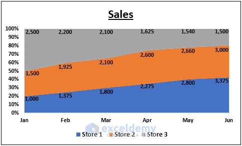
- Assume you have the following dataset. It contains the monthly sales made by different stores.

📌 Step 2: Insert Area Chart
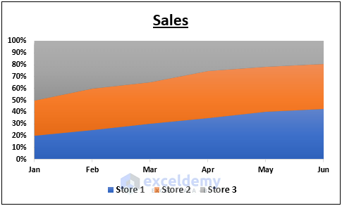
- Now click anywhere in the dataset first to insert an area chart. Then select Insert >> Insert Line or Area Chart. Next, choose a chart type from the list of 2-D Area or 3-D Area. Here, we will insert a 2-D 100% Stacked Area Chart.

- After that, you will get the following result. But the area chart is not showing the data labels.

Read More: Excel Stacked Area Chart Negative Values
📌 Step 3: Show Data Labels
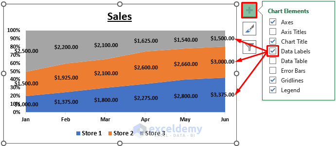
- Now click on the Chart Element menu and check the Data Labels checkbox. After that, the data labels will be visible. But the data labels overlap the axes.
📌 Step 4: Format Data Labels
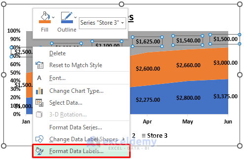
- Now right-click on a data label and select Format Data Labels. This will format the data labels of that particular data series only.
- Now uncheck Show Leader Lines. Then, change the number category from General to Number. Next, enter 0 for Decimal Places. Now repeat this for the data labels of each of the data series.

- After that, you will get the following result. Now it will be easier to fix the data label position in the area chart.

Read More: Stacked Area Chart with Line in Excel
📌 Step 5: Change Data Label Position
- Now click twice on a data label to select that particular data label. Then drag the data label to the desired position as shown below. Next, do this for each of the data labels.
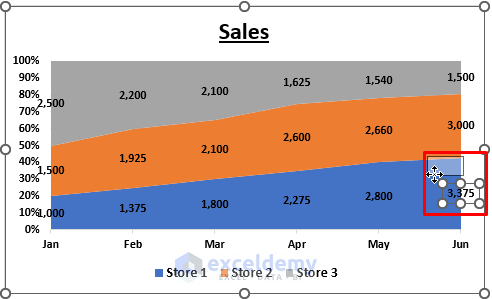
- Finally, you will see the following result.
Things to Remember
- You need to select the chart to access the Chart Element menu and other chart editing options.
- Hold the SHIFT key to drag the data labels horizontally or vertically.
- You can use Microsoft Power BI to automatically adjust the data label position in the area chart.
Download Practice Workbook
You can download the practice workbook from the download button below.
Conclusion
Now you know how to fix the Excel area chart data label position. Do you have any further queries or suggestions? Please let us know using the comment section below. You can also visit our ExcelDemy blog to explore more about Excel. Stay with us and keep learning.
Related Articles
- Proportional Area Chart Excel
- Smooth Area Chart Excel
- How to Shade an Area of a Graph in Excel
- Excel Area Chart X-axis Scale
- Excel Stacked Area Chart Change Order
- Excel Stacked Area Chart with Line
<< Go Back To Excel Area Chart | Excel Charts | Learn Excel
Get FREE Advanced Excel Exercises with Solutions!
