Watch Video – Create an Area Chart in Excel
Example 1 – Make a Simple 2-D Area Chart in Excel
Steps:
- Select range B6:E12.
Cell B6 is the first cell of the column Week and cell E12 is the last cell of the column MacBook Pro 16.
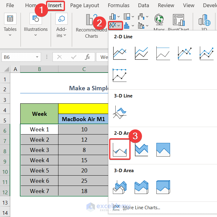
- Go to the Insert tab.
- Select Insert Line or Area Chart.
- Click on Area to insert a simple Area Chart.
To format the chart and add elements.
- Right-click on the chart.
- Click on Select Data.
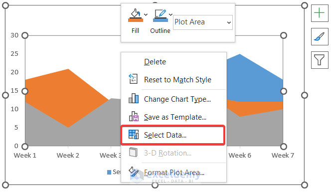
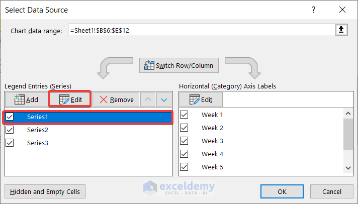
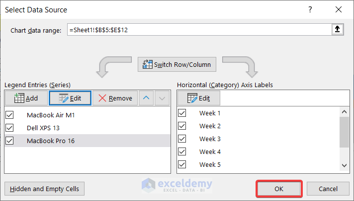
- A Select Data Source box will open.
- Select Series 1 from the Legend Entries (Series).
- Click on Edit.
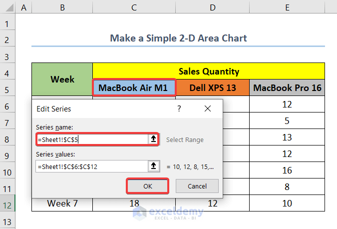
- In the Series name insert the cell C5 which indicates the name of the model MacBook Air M1.
- Click on OK.
- Change Series 2 to Dell XPS 13 and Series 3 to MacBook Pro 16.
- Click OK.
- Select the chart.
- Click on Chart Elements.
- Check the box for Axis Titles.
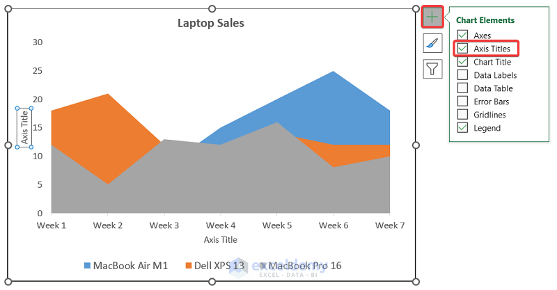
- Double-click on the Axis Titles to edit the text.
- Change the X-axis title to Sales Quantity and the Y-axis title to Week.
Note: You can add other chart elements to the chart like Data Labels or Data Table.
- You will have your simple 2-D Area Chart as shown in the image below.

Read More: How to Shade an Area of a Graph in Excel
Example 2 – Create a Stacked 2-D Area Chart in Excel
Steps:
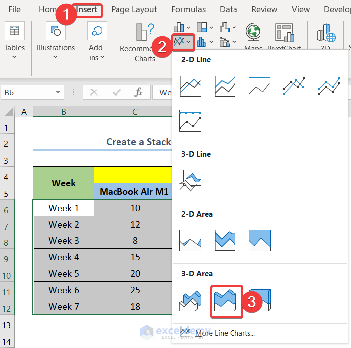
- Select range B6:E12.
- Go to the Insert tab.
- Select Insert Line or Area Chart.
- Click on Stacked Area to insert a Stacked Area Chart.
- Format and add elements to the chart.

Read More: Excel Stacked Area Chart Negative Values
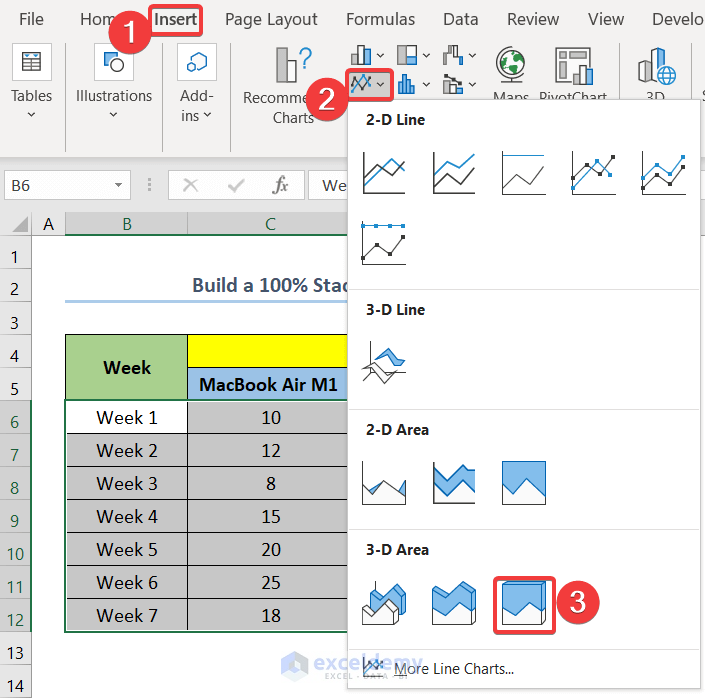
Example 3 – Build a 100% Stacked 2-D Area Chart in Excel
Steps:
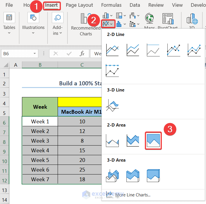
- Select range B6:E12.
- Go to the Insert tab.
- Select Insert Line or Area Chart.
- Click on 100% Stacked Area to insert a 100% Stacked Area Chart.
- Format and add elements to the chart.

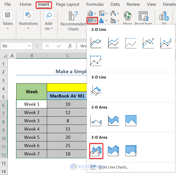
Example 4 – Make a Simple 3-D Area Chart in Excel
Steps:
- Select range B6:E12.
- Go to the Insert tab.
- Select Insert Line or Area Chart.
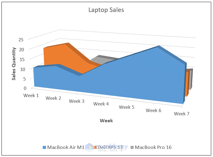
- Click on 3-D Area to insert a simple 3-D Area Chart.
- Format and add elements to the chart.
Example 5 – Create a Stacked 3-D Area Chart in Excel
Steps:
- Select range B6:E12.
- Go to the Insert tab.
- Select Insert Line or Area Chart.
- Click on 3-D Stacked Area to insert a 3-D Stacked Area Chart.
- Format and add elements to the chart.

Read More: Excel Area Chart Data Label Position
Example 6 – Build a 100% Stacked 3-D Area Chart in Excel
Steps:
- Select range B6:E12.
- Go to the Insert tab.
- Select Insert Line or Area Chart.
- Click on 3-D 100% Stacked Area to insert a 3-D 100% Stacked Area Chart.
- Format and add elements to the chart.

Things to Remember
- In a 100% Stacked Area Chart, you will get the percentage of total sales for a week for each model. To read this chart for Week 1, see the Y-Axis value for MacBook Air M1, which is 25%. Above the MacBook Air M1, the sales percentage of Dell XPS 13 is stacked, which will be at (25+45)%=70%. The rest of the sales percentage is for MacBook Pro 16.
- You can read the values for a Stacked Area Chart. In this case, the Y-axis represents the direct values of sales quantity.
- You can change the order for Excel Stacked Area Charts using the Select Data Source box.
Download Practice Workbook
Related Articles
<< Go Back To Excel Area Chart | Excel Charts | Learn Excel
Get FREE Advanced Excel Exercises with Solutions!
