How to Change the Order of an Excel Stacked Area Chart (With Quick Steps)

How to Add a Stacked Area Chart in Excel

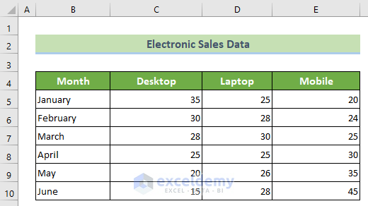
We have a dataset of 6 months’ sales data of an electronic store. Using these data, you can create a stacked area chart in Excel by following the steps below.

Steps:

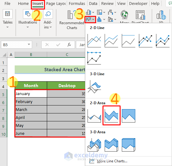
• Select your dataset, which is B5:E10 here.
• Go to the Insert tab >> Insert Line or Area Chart tool >> Stacked Area option.

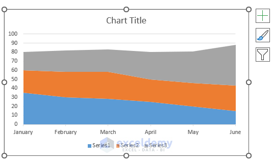
• You will see a stacked area chart for your selected data range.

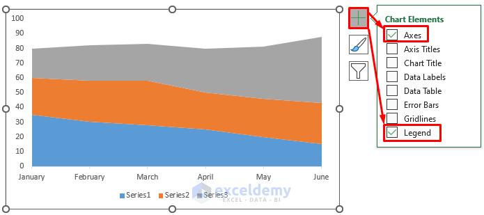
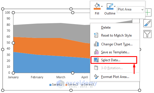
• To visualize the chart better, click on the Chart Elements tool and tick only the Axes and Legend options.

• To clarify the chart, right-click on the chart area and choose the Select Data… option from the context menu.

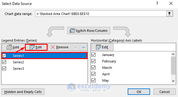
• The Select Data Source window will appear.
• Click on the Series 1 legend entry and click on the Edit button.

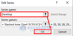
• The Edit Series window will appear now.
• Type ‘Desktop’ in the Series name: text box, as this dataset represents the Desktop column data.
• Click OK.

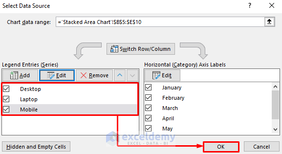
• For Series 2 and 3, write ‘Laptop’ and ‘Mobile’.
• Click on OK from the Select Data Source window.

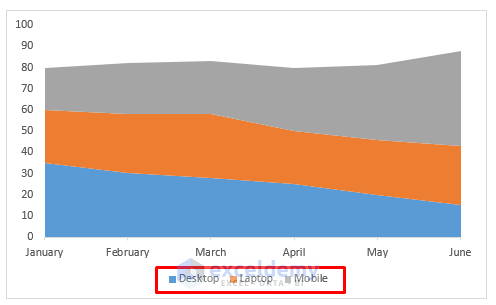
You can see you now have an understandable and better-looking stacked area chart of your dataset. It will look like this.

How to Change Order of Stacked Area Chart in Excel (With Easy Steps)

Step 1: Right-click on Chart Area and Navigate to Select Data Source Window

• Click on the chart area and right-click.
• Choose the Select Data… option from the context menu.

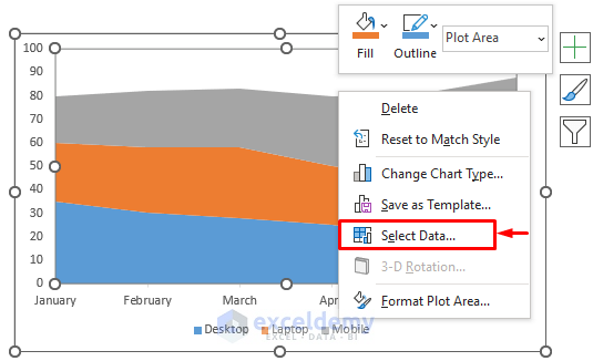
• The Select Data Source window will appear.

Read More: Excel Stacked Area Chart Negative Values

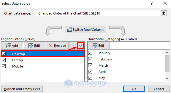
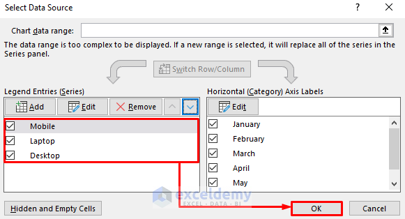
Step 2: Reorganize the Order of the Series

• Select the Desktop series and click the downward arrow button twice.

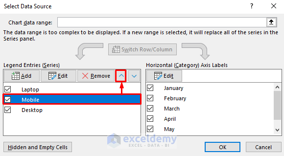
• Select the Mobile series and click on the upward arrow button.

Read More: Excel Area Chart Data Label Position

Final Step: Finalize the Series Order

• Now, you can see that all the series are aligned as you want them.
• Click OK.

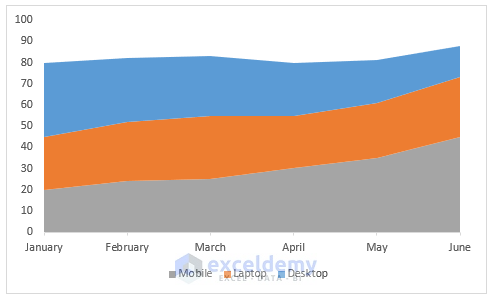
You can change the Excel stacked area chart order to your requirements. The outcome should look like this.

Download the Practice Workbook

You can download and practice from our workbook here.

Related Articles

• Proportional Area Chart Excel
• Smooth Area Chart Excel
• How to Shade an Area of a Graph in Excel

<< Go Back To Excel Area Chart | Excel Charts | Learn Excel