What-If Analysis in Excel with Examples: Complete Guide

Method 1 – What-If Analysis of House Rent in Excel

Our first example is based on the house rent. Using the scenario manager, you can find out which house is applicable for us. We would like to consider two scenarios

• House 2
• House 3

The initial condition or dataset can consider as house 1. The scenario manager summary will give us the total cost of each house. Using this summary, you can select any possible house to stay in. To understand the example clearly, follow the steps.

Steps

• We need to calculate the total cost of the initial dataset.
• Select cell C10.
• Write down the following formula using the SUM function.

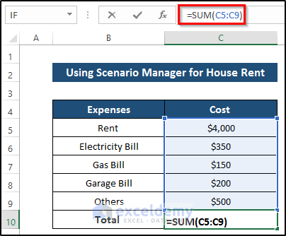
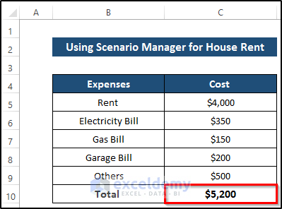
• Press Enter to apply the formula.

• Go to the Data tab in the ribbon.
• Select the What-If Analysis drop-down option from the Forecast group.
• Select the Scenario Manager option.

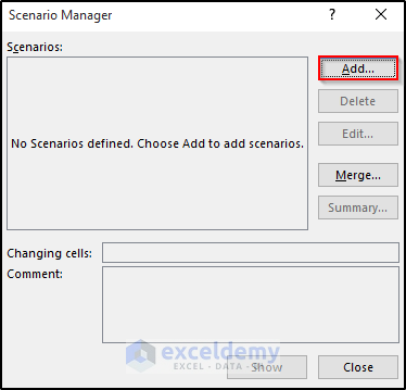
• Open the Scenario Manager dialog box.
• Select Add to include new scenarios.

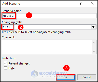
• The Add Scenario dialog box will appear.
• Set House 2 as the Scenario name.
• Set the range of cells C5 to C9 as the Changing cells.
• Click on OK.

• It will take us to the Scenario Values dialog box.
• Put the input values of rent, electricity bill, gas bill, garage bill, and others.

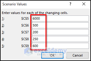
• Click on OK.
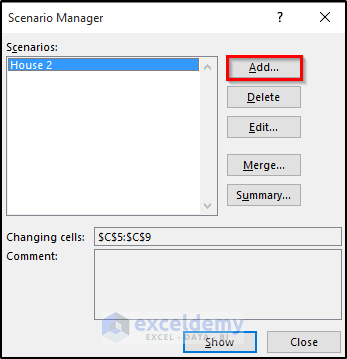
• It will take us back to the Scenario Manager dialog box.
• Click on Add to include another scenario.

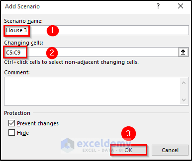
• The Add Scenario dialog box will appear.
• Set House 3 as the Scenario name.
• Set the range of cells C5 to C9 as the Changing cells.
• Click on OK.

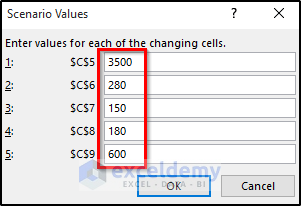
• It will take us to the Scenario Values dialog box.
• Put the input values of rent, electricity bill, gas bill, garage bill, and others.
• Click on OK.

• In the Scenario Manager dialog box, select Summary.

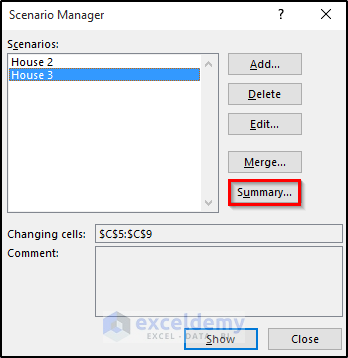
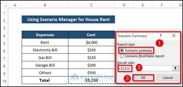
• The Scenario Summary dialog box will appear.
• Select Scenario Summary as Report Type.
• Set cell C10 as the Result cells.
• Click OK.

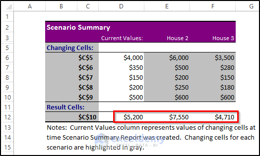
• Get the following results where you get the outcome without creating a new worksheet.

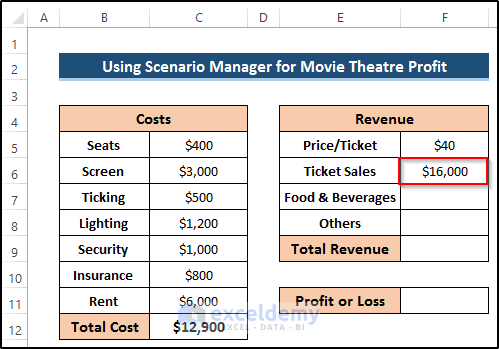
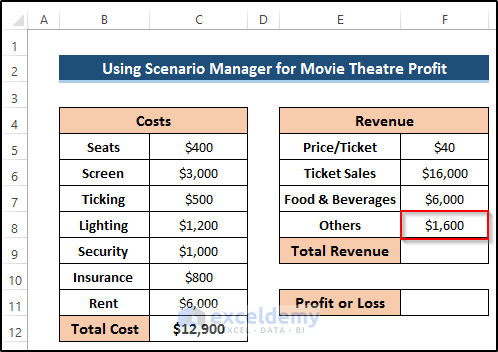
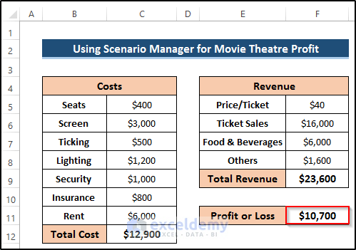
Method 2 – Performing What-If Analysis for Movie Theatre Profit

Our next example is based on the scenario of the movie theatre. We will focus on the profit of movie theatres for different scenarios. Take a dataset that consists of the cost and revenue of a small movie theatre. We would like to use the scenario manager to get the final output for several scenarios.

We would like to take two scenarios under consideration.

• Medium Venue
• Large Venue

To use a what-if analysis scenario manager for a movie theater example, follow the steps carefully.

Step 1: Calculate Movie Theatre Profit

We need to calculate the revenue amounts. The cost of the movie theatre changes with its size. Utilize the scenario manager in that case. To calculate the movie theater profit, follow the following steps.

• Select cell F6 to calculate the Ticket Sales.
• Write down the following formula.

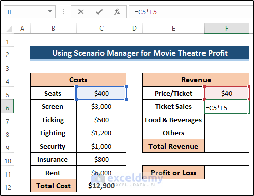
• Press Enter to apply the formula.

• Select cell F7 to calculate the Food & Beverages.
• We create a link with the total number of seats in the movie theater. By using the total number of seats, we assume the Food & Beverages amount.
• Write down the following formula.

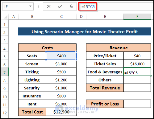
• Press Enter to apply the formula.

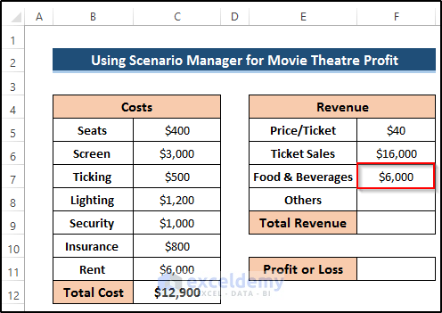
• Select cell F8 to calculate the Others.
• We create a link with the total number of seats in the movie theatre. By using the total number of seats, we assume the Others amount.
• Write down the following formula.

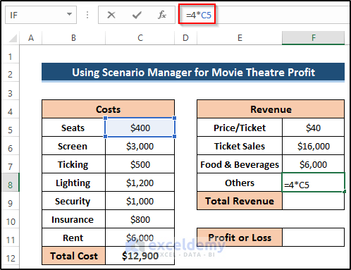
• Press Enter to apply the formula.

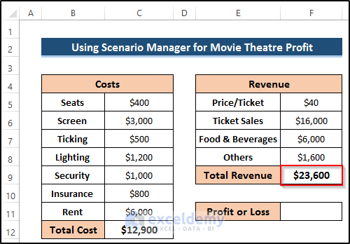
• To calculate the Total Revenue, select cell F9.
• Write down the following formula using the SUM function.

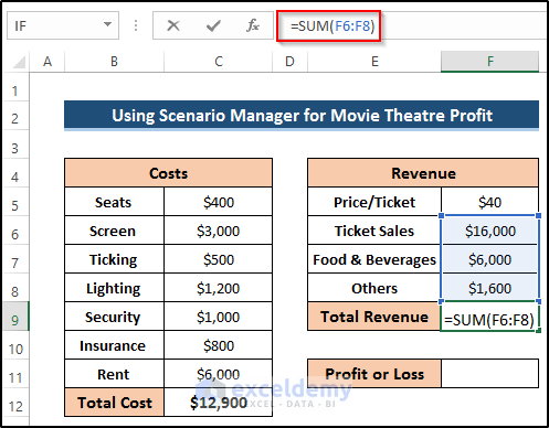
• Press Enter to apply the formula.

• Calculate the profit earned by the movie theatre.
• Select cell F11.
• Write down the following formula.

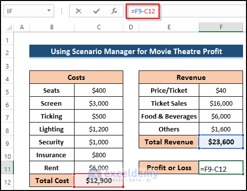
• Press Enter to apply the formula.

Step 2: Create Scenarios

Create three different scenarios in the Scenario Manager. These three scenarios include medium venue, large venue, and very large venue. To create these, follow the steps.

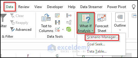
• Go to the Data tab in the ribbon.
• Select the What-If Analysis drop-down option from the Forecast group.
• Select the Scenario Manager option.

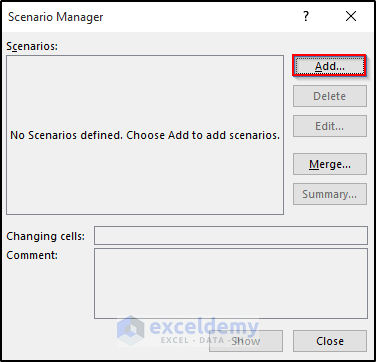
• Open the Scenario Manager dialog box.
• Select Add to include new scenarios.

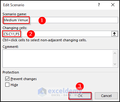
• The Edit Scenario dialog box will appear.
• Set Medium Venue as Scenario name.
• Select the range of cells C5 to C11 and cell F5. That means all the cost changes along with the size of the theater. Ticket prices will also increase.
• Click OK.

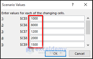
• It will open up the Scenario Values dialog box.
• Set values for a medium venue. In this section, we need to change the seats, ticketing, lighting, security, insurance, rent, and ticket price.

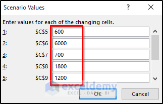
• Scroll down and set another cell value properly. See the screenshot.

• Click on OK.
• It will take us to the Scenario Manager dialog box again.
• Select Add to include another scenario.

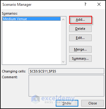
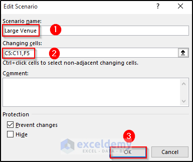
• Set Large Venue as the Scenario name.
• Select range of cell C5 to C11 and cell F5. That means all the cost changes along with the size of the theater. Ticket prices will also increase.
• Click OK.

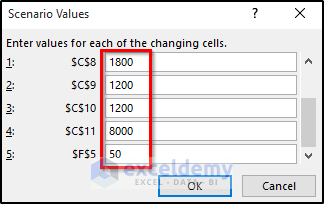
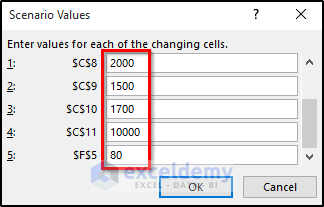
• It will open up the Scenario Values dialog box.
• Set values for a large venue. Change the seats, ticketing, lighting, security, insurance, rent, and ticket price.

• Scroll down and set another cell value properly. See the screenshot.
• Click OK.

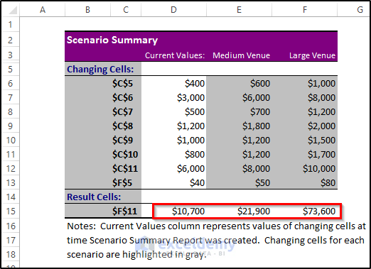
Step 3: Generate Scenario Summary

Create a summary of the scenarios including the initial one. The summary includes the input values and the estimated output of the created scenarios.

• In the Scenario Manager dialog box, select the Summary.

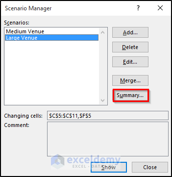
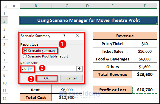
• The Scenario Summary dialog box will appear.
• Select Scenario Summary as Report Type.
• Set cell F11 as the Result cells.
• Click on OK.

• Get the summary of all the scenarios including the initial one.
• This summary implies how the profit changes with the size of the theater.
• It also helps us to think about the cost section more and how to utilize and get the best possible solution.

Examples of What-If Analysis Using Goal Seek in Excel

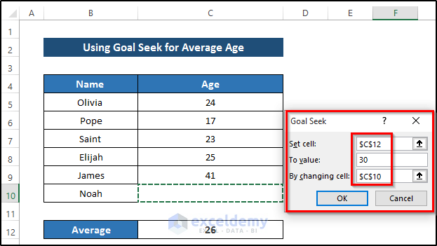
Method 1 – Using Goal Seek for Average Age

Steps

• Calculate the average using the available dataset.
• Select cell C12.
• Write down the following formula using the AVERAGE function.

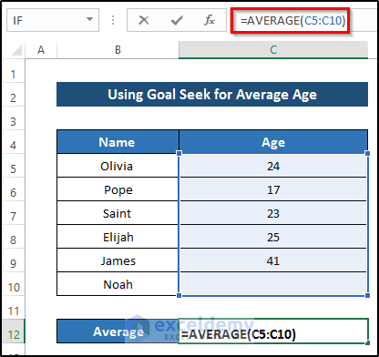
• Press Enter to apply the formula.

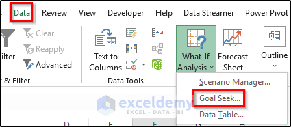
• Go to the Data tab on the ribbon.
• Select What-If Analysis drop-down option.
• Select Goal Seek from the What-If Analysis drop-down option.

• The Goal Seek dialog box will appear.
• Put cell C12 in the Set Cell section.
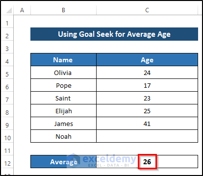
• Put 30 in the To value section.
• Set cell C10 in the By changing cell section.

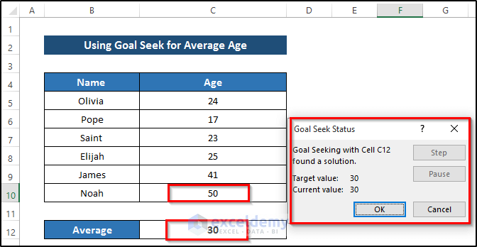
• Get the Goal Seek Status dialog box where it denotes that they get a solution.
• Find the change in the Average and input value of a certain cell.

Method 2 – What-If Analysis for Exam Marks

Steps

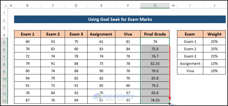
• Calculate the final grade of each student using exam marks and the weight of each exam.
• Select cell G5.
• Write down the following formula in the formula box.

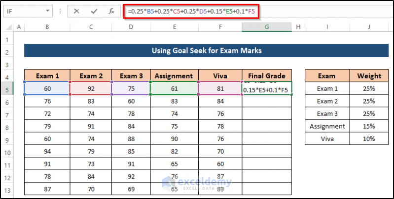
• Press Enter to apply the formula.

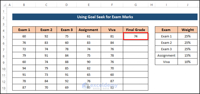
• Drag the Fill Handle icon down the column.

• Go to the Data tab on the ribbon.
• Select What-If Analysis drop-down option.
• Select Goal Seek from the What-If Analysis drop-down option.

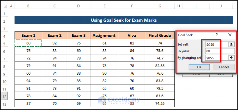
• The Goal Seek dialog box will appear.
• Put cell G5 in the Set Cell Section.
• Put 80 in the To value Section.
• Set cell B5 in the By changing cell Section.

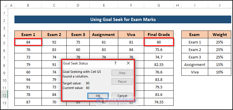
• Get the Goal Seek Status dialog box where it denotes that they get a solution.
• Find the change in the Final Grade as 80 and the input value of Exam 1 becomes 84.

Examples of What-If Analysis Using Data Table in Excel

Method 1 – Calculating EMI with One Dimensional Approach

Steps

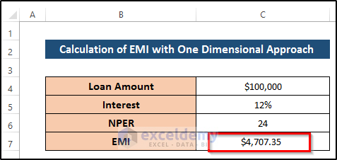
• Calculate the initial EMI using the given dataset.
• Select cell C7.
• Write down the following formula using the PMT function.

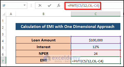
• Press Enter to apply the formula.

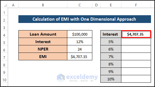
• Set two new columns and put all the interest rates.
• Put the calculated EMI value in the next column.

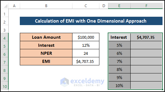
• Select the range of cells E4 to F10.

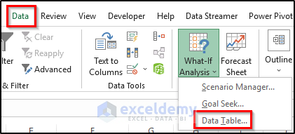
• Go to the Data tab on the ribbon.
• Select What-If Analysis drop-down option from the Forecast group.
• Select Data Table from What-If Analysis drop-down option.

• The Data Table dialog box will appear.
• Set cell C5 as the Column input cell.

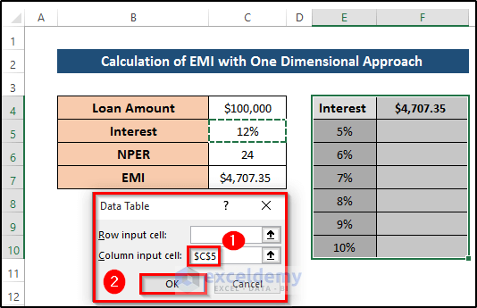
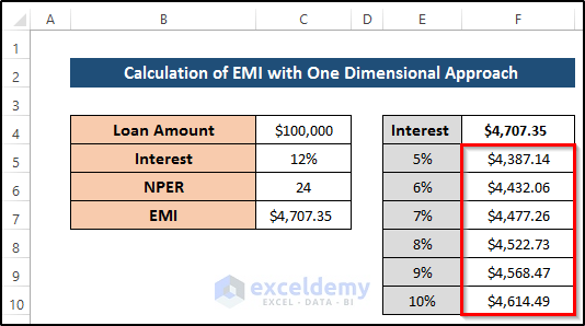
• You will see the EMI values are calculated for different interest rates. See the screenshot.

Method 2 – Calculating EMI with Two Dimensional Approach

Steps

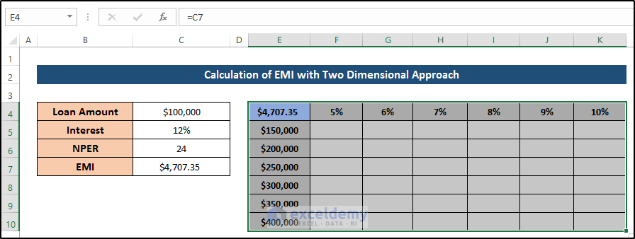
• Calculate the initial EMI using the given dataset.
• Select cell C7.
• Write the following formula.

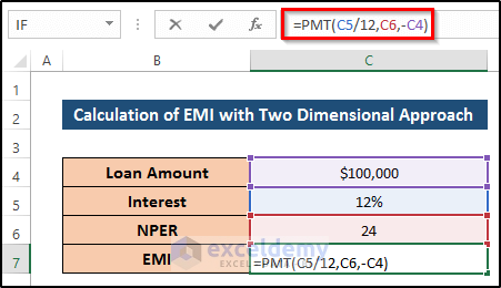
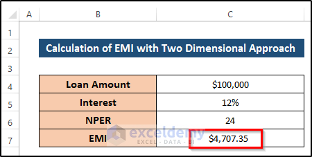
• Press Enter to apply the formula.

• Create several columns that include different interest rates and loan amounts.

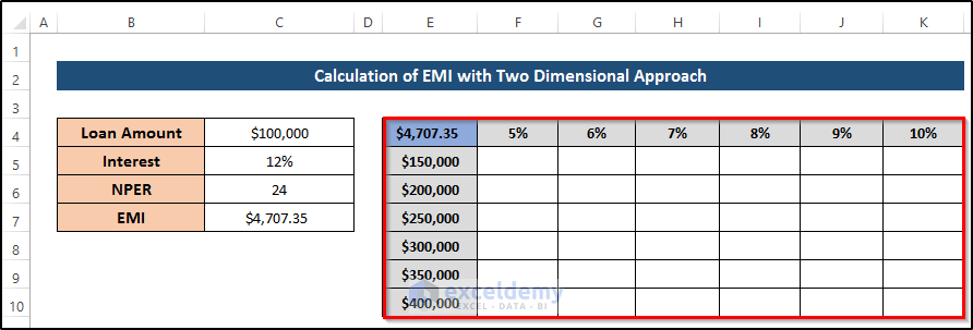
• Select the range of cells E4 to K10.

• Go to the Data tab on the ribbon.
• Select What-If Analysis drop-down option from the Forecast group.
• Select Data Table from What-If Analysis drop-down option.

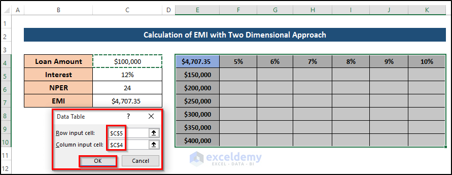
• The Data Table dialog box will appear.
• Set cell C5 means the Interest Rate as Row input cell.
• Set cell C4 means the Loan Amount as Column input cell.
• Click OK.

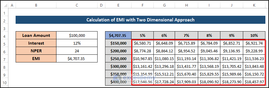
• See the EMI values are calculated for different interest rates and loan amounts. See the screenshot.

Things to Remember

• The scenario summary report can’t automatically recalculate. So, if you change the dataset, there will be no change in the summary report.
• You don’t require result cells to generate a scenario summary report, but you need to require them for a scenario PivotTable report.
• Check the goal-seeking parameters. The supposed output cell must contain a formula that depends on the supposed input values.
• Try to avoid circular reference in both formula and goal-seeking parameters.

Download Practice Workbook

Download the practice workbook below.

Related Articles

• How to Delete What If Analysis in Excel
• What If Analysis Data Table Not Working
• How to Build a Sensitivity Analysis Table in Excel
• How to Do IRR Sensitivity Analysis in Excel

<< Go Back to What-If Analysis in Excel | Learn Excel