In this article, I’ll show you the step-by-step process of how to calculate the standard error of skewness in Excel. Apart from this, I’ll discuss the relevant topics also.
What Is Skewness and Standard Error?
Skewness represents the degree of asymmetry in a given set of data. In a distribution, when the tail on the left side is longer, you may say that the distribution is negatively skewed (left-skewed). On the contrary, a distribution will be positively skewed (right-skewed) if the tail on the right side is longer than on the left side.
Besides, the standard error (SE) denotes the variability of the given dataset. Mainly, it is the standard deviation of the sampling distribution. The formula for calculating the SE is as follows-
SE=Standard Deviation/NWhere N is the sample size.
What Is Standard Error of Skewness (SES)?
You can determine the standard error of skewness (SES) when the value of skewness is so large. The SES is mainly the ratio of skewness regarding the standard error of the given dataset. However, the standard value of the SES lies between -2 to +2.
Let’s look at the following equation for calculating the standard error of skewness (SES).
SES=6*N*(N-1)/(N-1)*(N+1)*(N+3)Where N is the sample size.
How to Calculate Skewness in Excel
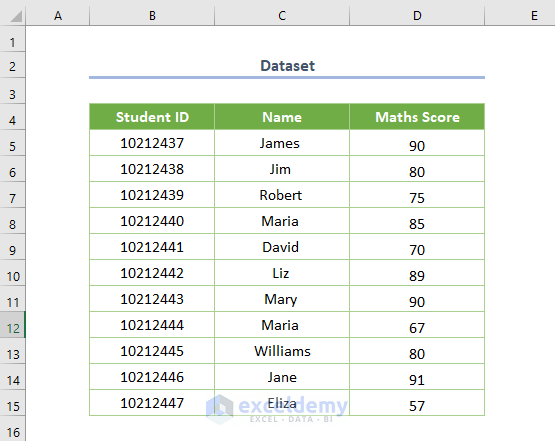
Let’s have a look at the following dataset where Maths Score is given along with Student ID and Student’s Name.
Now, let’s move on to the methods.
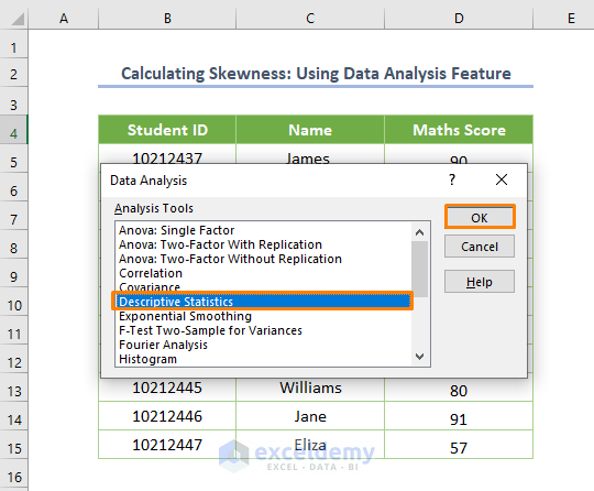
1. Using Data Analysis Feature
To calculate using the Data Analysis feature please do the following steps.
- Firstly, enable the Data Analysis feature if you don’t find it in the Data tab.
- Then, click on the added Data Analysis feature and choose the Descriptive Statistics option. And press OK.
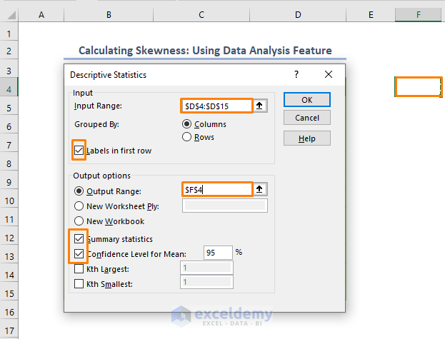
- Now, specify the Input Range as $D$4:$D$15, and the Output Range as $F$4. Besides, check the boxes before the Labels, Summary statistics, or other relevant options.
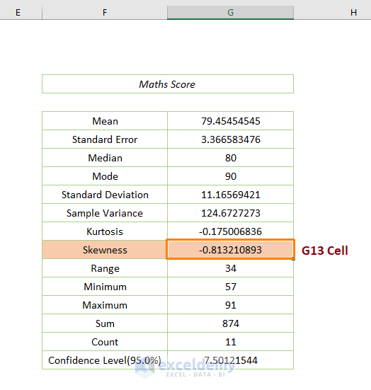
Eventually, you’ll get the skewness in the G13 cell of the file as -0.813.
Read More: How to Calculate Standard Error in Excel
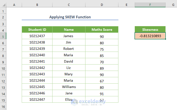
2. Applying SKEW Function
In addition, you can apply the SKEW function to find the skewness of the Maths Score.
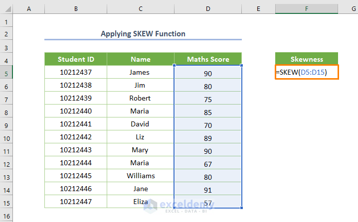
Just insert the following formula.
=SKEW(D5:D15)
Here, D5:D15 is the cell range representing Math Scores.
After pressing the ENTER key, you’ll get the same output as found in the first method which is -0.813.
How to Calculate Standard Error in Excel
Here, I’ll discuss 2 simple methods to determine the standard error in Excel.
1. Using Data Analysis Feature
If you look closely at the output found in the first method of calculating skewness, you’ll see the value of the standard error in the G7 cell.

Read More: How to Calculate SEM in Excel
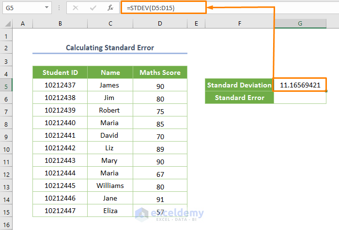
2. Utilizing Excel Functions
Luckily, you can utilize Excel functions to determine the standard error in Excel.
Initially, you need to calculate the standard deviation. For example, use the following formula.
=STDEV(D5:D15)
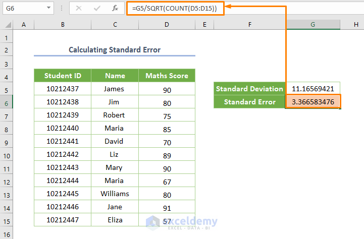
Next, you have to utilize the following formula.
=G5/SQRT(COUNT(D5:D15))
⧬ Formula Explanation:
Here, the COUNT function counts the number of sample sizes first. Later, the SQRT function returns the square root of the number of the size. Lastly, divide the standard deviation by the square root of the sample sizes.
How to Calculate Standard Error of Skewness in Excel
If you need to calculate the SES in Excel, you may follow the two steps.
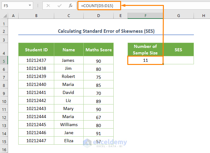
Step 01: Find the Number of Sample Size
Firstly, you need to count the number of a given dataset. You can use the below formula.
=COUNT(D5:D15)
Step 02: Calculate SES with the Formula
By the time you’re exploring this section, you’ve known the formula to calculate SES (I’ve discussed earlier). If you have a closer look at the formula, you can see I need to square root the result. To do that you can apply the SQRT function. The entire formula will be like the following-
=SQRT((6*F5*(F5-1))/((F5-2)*(F5+1)*(F5+3)))
Here, F5 is the number of sample sizes.

As the value of the SES is 0.66, you can say that this is a standard value and the sample distribution is non-symmetric (right-skewed). Further, you can multiply 1.96 by the value of SES to get the margin of error.
Read More: How to Calculate Standard Error of Regression in Excel
Download Practice Workbook
Conclusion
This is how you can calculate the standard error of skewness in Excel. I firmly believe this article will be highly beneficial for you. Anyway, don’t forget to share your thoughts.
Related Articles
- How to Find Residual Standard Error in Excel
- How to Calculate Standard Error of Regression Slope in Excel
- How to Calculate Standard Error of Proportion in Excel
- How to Calculate Standard Error of Correlation Coefficient in Excel
- How to Find Standard Error of Estimate in Excel
<< Go Back to Standard Error in Excel | Excel for Statistics | Learn Excel
Get FREE Advanced Excel Exercises with Solutions!
