We use regression analysis when we have data from two variables from two different sources and want to build a relationship between them. Regression analysis provides us with a linear model that allows us to predict possible outcomes. There will be some differences between the predicted and actual values for obvious reasons. As a result, we calculate the standard error using the regression model, which is the average error between predicted and actual values. In this tutorial, we will show you how to calculate the standard error of regression analysis in Excel.
Calculate Standard Error of Regression in Excel: 4 Simple Steps
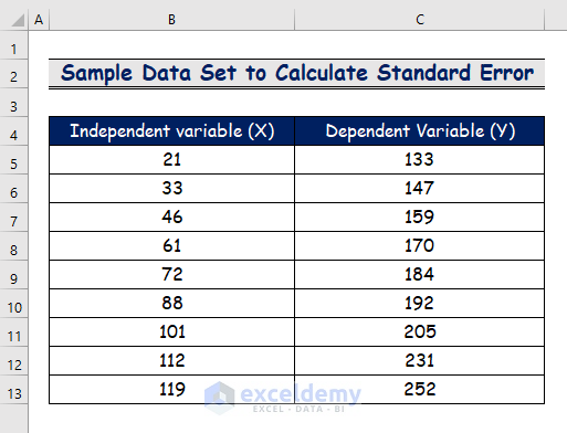
Assume you have a data set with an independent variable (X) and a dependent variable (Y). As you can see, they have no significant relationship. But we want to build one. As a result, we’ll use Regression Analysis to create a linear relationship between the two. We’ll calculate the standard error between the two variables using the regression analysis. We’ll go over some of the regression model’s parameters in the second half of the article to help you interpret it.
Step 1: Apply Data Analysis Command to Create a Regression Model
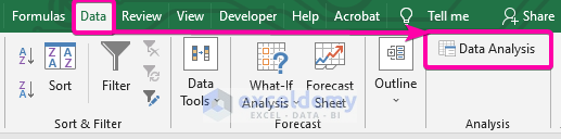
- Firstly, go to the Data tab and click on the Data Analysis command.
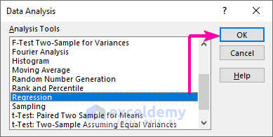
- From the Data Analysis list box, select the Regression option.
- Then, click OK.
Step 2: Insert Input and Output Range in Regression Box
- For the Input Y Range, select the range C4:C13 with the header.
- Click on the Labels check box.
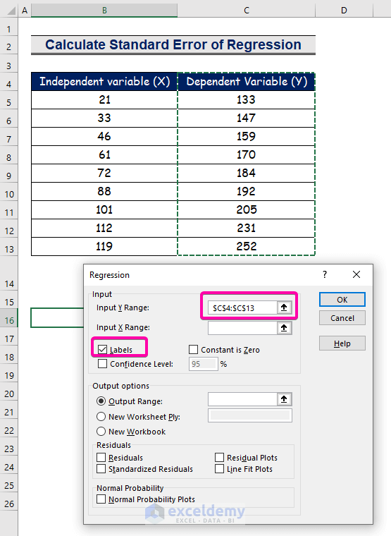
- Select the range B4:B13 for the Input X Range.
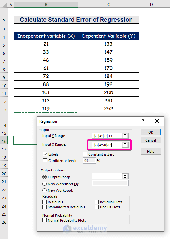
- To get the result in the preferred location, select any cell (B16) for the Output Range.
- Finally, click OK.

Read More: How to Calculate Standard Error in Excel
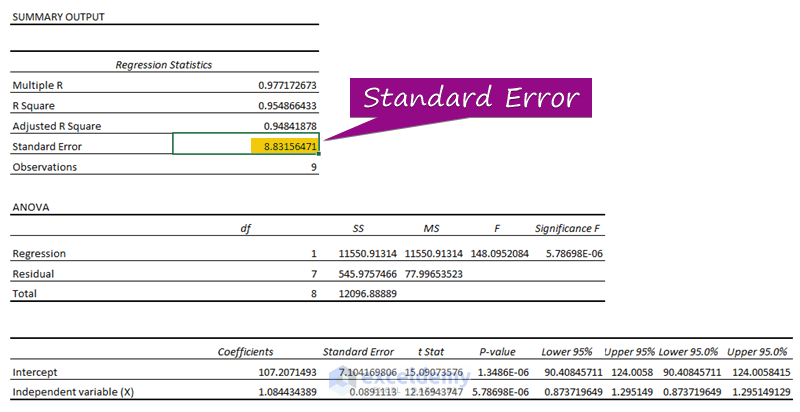
Step 3: Find Out Standard Error
- From the regression analysis, you can obtain the value of the standard error (3156471).
Read More: How to Calculate SEM in Excel
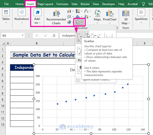
Step 4: Plot Regression Model Chart
- Firstly, click on the Insert tab.
- From the Charts group, select the Scatter chart.
- Right-click over one of the points.
- From the options, select the Add trendline option.
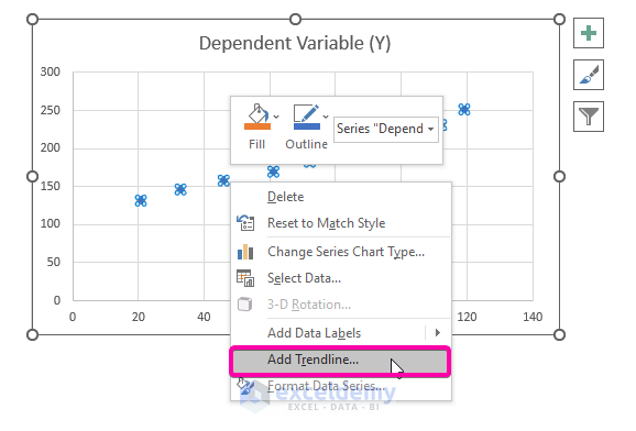
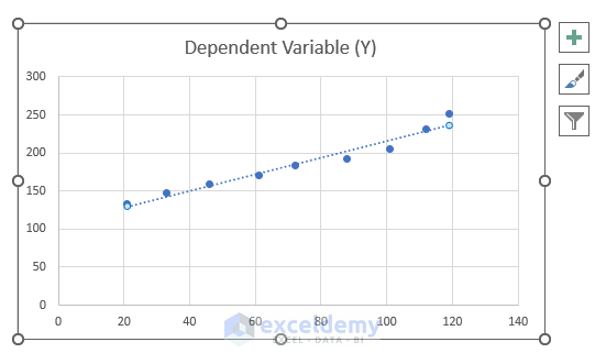
- Therefore, your regression analysis chart will be plotted as the image shown below.
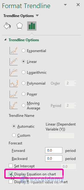
- To display the regression analysis equation, click on the Display equation on Chart option from the Format Trendline.
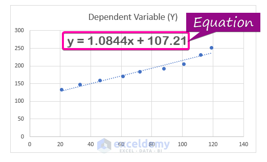
- As a result, the equation (y = 1.0844x + 107.21) of the regression analysis will appear in the chart.
Notes:
You can calculate the difference between the predicted values and the actual values from the equation of regression analysis.
Steps:
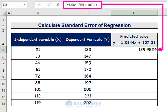
- Type the formula to represent the regression analysis equation.
=1.0844*B5 + 107.21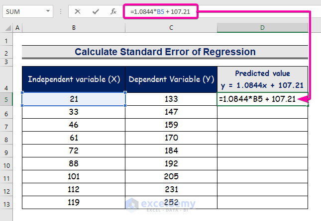
- Therefore, you will get the first predicted value (129.9824), which differs from the actual value (133).
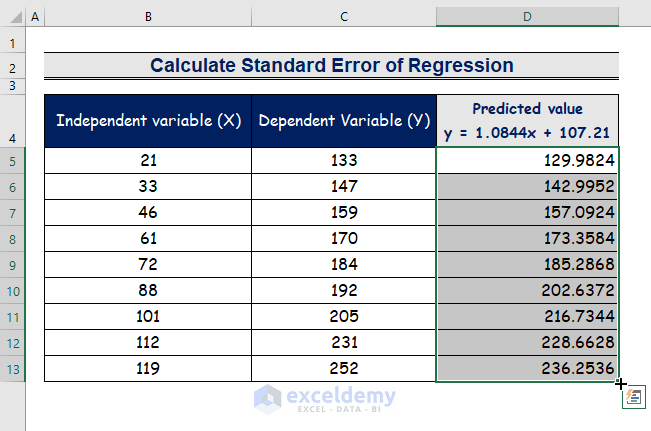
- Use the AutoFill Tool to auto-fill column D.
- To calculate the error, type the following formula to subtract.
=C5-D5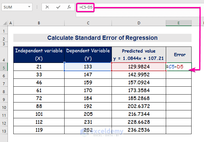
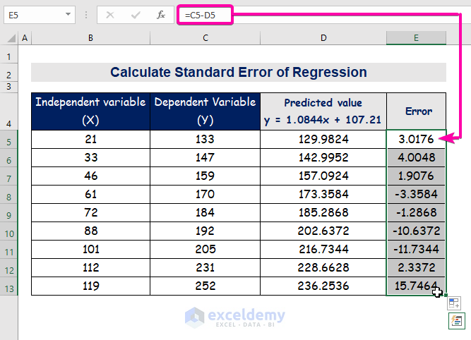
- Finally, auto-fill column E to find the error values.
Read More: How to Calculate Standard Error of Regression Slope in Excel
The Interpretation of Regression Analysis in Excel
1. Standard Error
We can see from the regression analysis equation that there is always a difference or error between the predicted and actual values. As a result, we must calculate the average deviation of the differences.
A standard error represents the average error between the predicted value and the actual value. We discovered 8.3156471 as the standard error in our example regression model. It indicates that there is a difference between the predicted and actual values, which could be greater than the standard error (15.7464) or less than the standard error (4.0048). However, our average error will be 8.3156471, which is the standard error.
As a result, the model’s goal is to reduce the standard error. The lower the standard error, the more accurate the model.
2. Coefficients
The regression coefficient evaluates the responses of unknown values. In the regression equation (y = 1.0844x + 107.21), 1.0844 is the coefficient, x is the predictor-independent variable, 107.21 is the constant, and y is the response value for the x.
- A positive coefficient predicts that the higher the coefficient, the higher the response variable. It indicates a proportional relationship.
- A negative coefficient predicts that the higher the coefficient, the lower the response values. It indicates a disproportional relationship.
3. P-Values
In regression analysis, p-values and coefficients cooperate to inform you whether correlations in your model are statistically relevant and what those relationships are like. The null hypothesis that the independent variable has no link with the dependent variable is tested using the p-value for each independent variable. There is no link between changes in the independent variable and variations in the dependent variable if there is no correlation.
- Your sample data gives enough support to falsify the null hypothesis for the full population if the p-value for a variable is less than your significance threshold. Your evidence supports the notion of a non-zero correlation. At the population level, changes in the independent variable are linked to changes in the dependent variable.
- A p-value larger than the significance level, on either side, suggests that your sample has insufficient proof to establish that a non-zero correlation exists.
Because their p-values (5.787E-06, 1.3E-06) are less than the significant value (5.787E-06), the Independent Variable (X) and Intercept are statistically significant, as seen in the regression output example.
4. R-Squared Values
For linear regression models, R-squared is a completeness measurement. This ratio shows the percentage of variance in the dependent variable that the independent factors account for when taken together. On a handy 0–100 percent scale, R-squared quantifies the strength of the connection between your model and the dependent variable.
The R2 value is a measure of how well the regression model fits your data. The higher the number, the better feasible the model.
Download Practice Workbook
Download this practice workbook to exercise while you are reading this article.
Conclusion
I hope this article has given you a tutorial about how to calculate the standard error of regression in Excel. All of these procedures should be learned and applied to your dataset. Take a look at the practice workbook and put these skills to the test. We’re motivated to keep making tutorials like this because of your valuable support.
Please contact us if you have any questions. Also, feel free to leave comments in the section below. Stay with us and keep learning.
Related Articles
- How to Find Residual Standard Error in Excel
- How to Calculate Standard Error of Skewness in Excel
- How to Calculate Standard Error of Proportion in Excel
- How to Calculate Standard Error of Correlation Coefficient in Excel
- How to Find Standard Error of Estimate in Excel
<< Go Back to Standard Error in Excel | Excel for Statistics | Learn Excel
Get FREE Advanced Excel Exercises with Solutions!
