How to Add Second Vertical Axis in Excel Scatter Plot (3 Suitable Ways)

Get FREE Advanced Excel Exercises with Solutions!

In this tutorial, I am going to show you how to add a second vertical axis in Excel scatter plot. This is needed when plotting two variables on the same graph that have large variations in their individual range. Then what happens is that one of the variables is plotted in a way that becomes very hard to visualize. Adding an extra vertical axis helps greatly in this situation.

Table of Contents hide

Download Practice Workbook

3 Suitable Ways to Add Second Vertical Axis in Excel Scatter Plot

1. Insert Scatter Plot with Two Vertical Axis on Opposite Sides in Excel

2. Add Second Vertical Axis on Same Side in Excel Scatter Plot

3. Using Chart Format Tab to Add Second Vertical Axis

Conclusion

Download Practice Workbook

You can download the practice workbook from here.

Add Second Vertical Axis.xlsx

3 Suitable Ways to Add Second Vertical Axis in Excel Scatter Plot

When we create a chart, by default Excel creates a primary horizontal axis and a primary vertical axis. For simple datasets, this default option may be enough for us. But for more complex datasets, we require some extra methods. In this short tutorial, we are going to dive into those methods.

1. Insert Scatter Plot with Two Vertical Axis on Opposite Sides in Excel

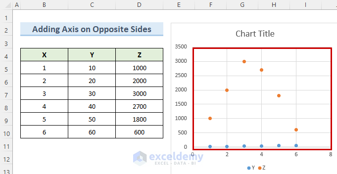
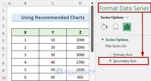
For this method, we have the following 3 variables data set. We have created a simple scatter plot using this dataset. As we can see, the variation of the Y variable is hard to spot. Let us add a vertical axis to this plot.

Steps:

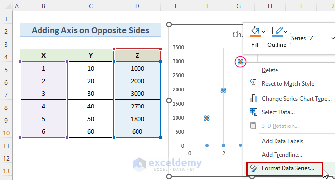
Firstly, right-click on the orange data series.
Now, from the context menu select Format Data Series.

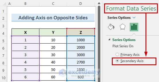
After that, in the new Format Data Series window, select Secondary Axis.

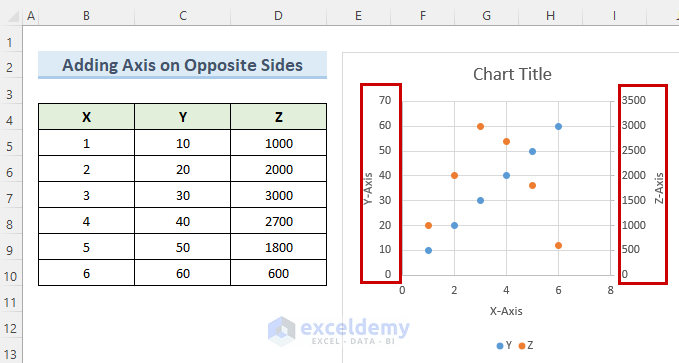
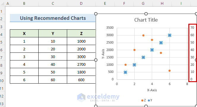
Finally, an additional vertical axis will be added to the chart, opposite to the first vertical axis.

2. Add Second Vertical Axis on Same Side in Excel Scatter Plot

This method actually takes the previous method a step forward. After creating an additional vertical axis, it can be positioned within clicks. Follow the steps below.

Steps:

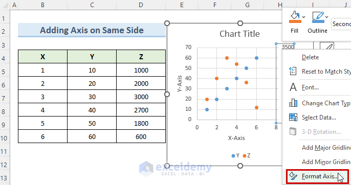
At the start, right-click on the newly added vertical axis.
Then, select Format Axis.

Now, in the opened Format Axis window, go to Labels.
Following this, select Low from the dropdown menu.

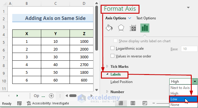
In the end, you should see your new vertical axis get positioned beside the old one.

3. Using Chart Format Tab to Add Second Vertical Axis

This method of adding a vertical axis is quite useful. It breaks down how Excel Chart formatting works on different data series. Let us apply this method in practice.

Steps:

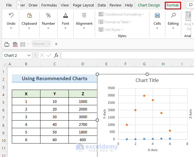
First of all, select your chart and go to the Format tab.
Note that, we can find this tab just beside the Chart Design tab.

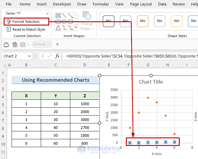
Now, click on the dropdown marked Chart Area.
Then, from this dropdown, select the Series Y option.

After doing that, the data series will be selected.
Now, select the Format Selection option. This will allow you to work with your selected data series.

Now, the Format Data Series window will open on the right side of your screen.
Then, inside this window, select the Secondary Axis option.

Finally, you will have a second vertical axis for your selected data series.

Conclusion

I hope that this tutorial was able to teach you multiple easy methods to add a second vertical axis in an Excel scatter plot. This technique is very helpful when you are working with datasets including multiple variables. You can extend the methods shown in this tutorial and add more variables to your data. Practicing will help you the most in understanding the steps. To learn more Excel techniques, follow our ExcelDemy website. If you have any queries, please let me know in the comments.