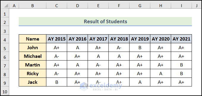
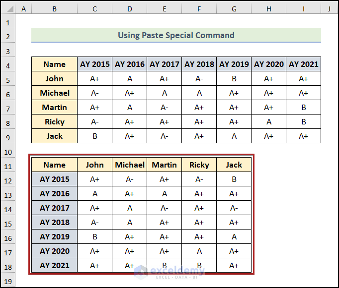
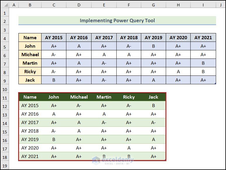
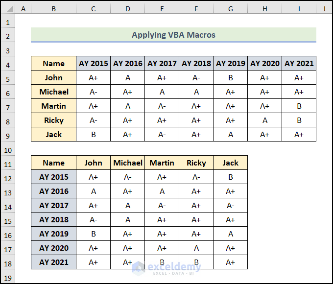
Below is a dataset that shows the year and Results of Students.
Method 1 – Using Paste Special Command
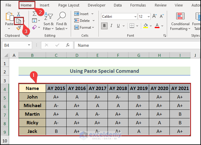
a) Pasting a Special Command from a Ribbon
Steps:
- Select cells in the B4:I9 range.
- Go to the Home tab.
- Click on the Copy icon on the Clipboard.
- Choose cell B11.
- Go to the Home tab.
- Click on the Paste drop-down icon on the Clipboard.
- Select Paste Special from the drop-down list.
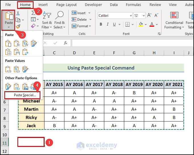
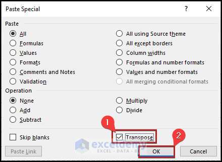
The Paste Special dialog box will pop up.
- Check Transpose.
- Click OK.
As a result, you see the new output in the B11:G18 range, which is the dataset’s transposed form.
b) Pasting From the Keyboard Shortcut
Steps:
- Select the whole dataset (B4:I9).
- Press CTRL + C.
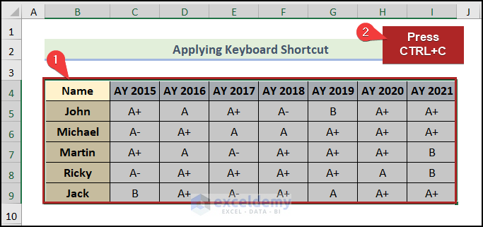
- Select cell B11 as the first cell of the destination range.
- Press CTRL + ALT + V.
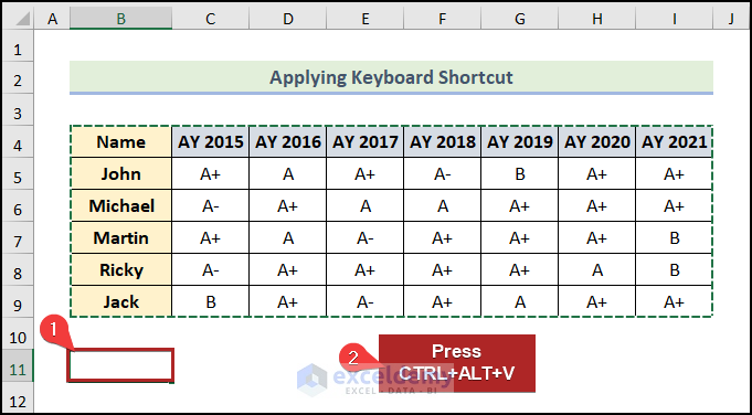
The Paste Special dialog box will open.
- Press E to check Transpose.
- Click OK or press ENTER.
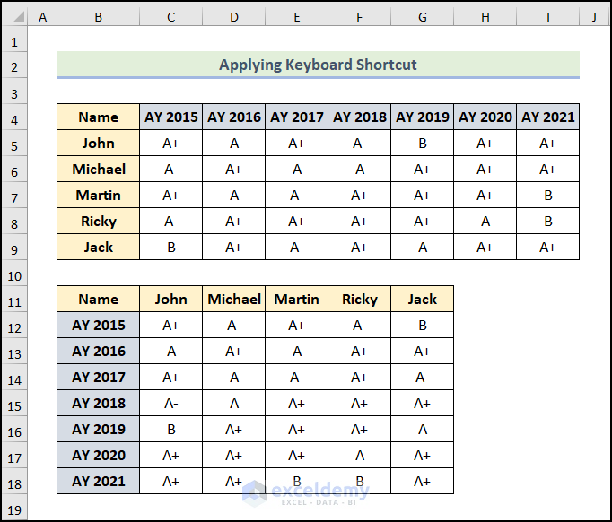
![]()
You see the transposed result.
Read More: How to Paste Transpose in Excel Using Shortcut (4 Easy Ways)
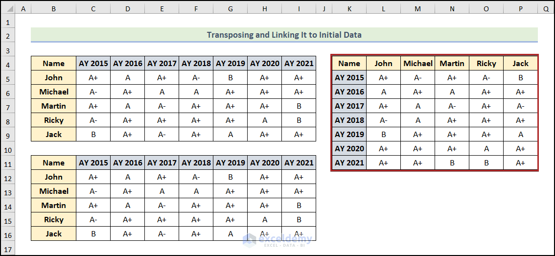
Method 2 – Transposing a Table and Linking It to the Initial Data
Steps:
- Select cells in the B4:I9 range.
- Press CTRL + C.
- Select cell B11.
- Press CTRL + ALT + V.
- Click on the Paste Link on the Paste Special wizard.
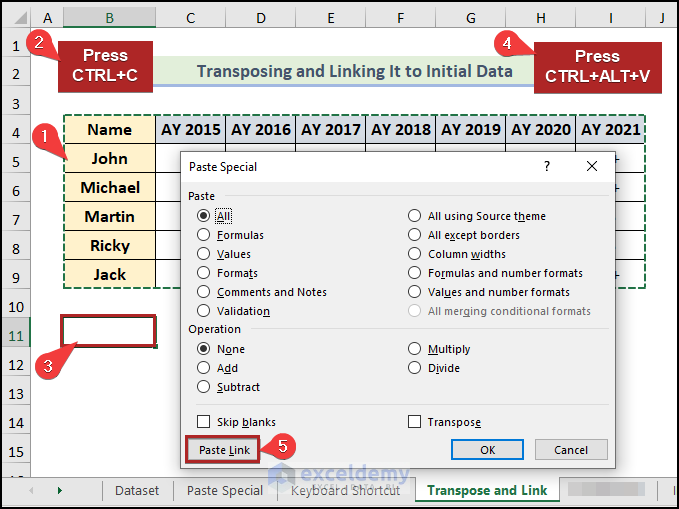
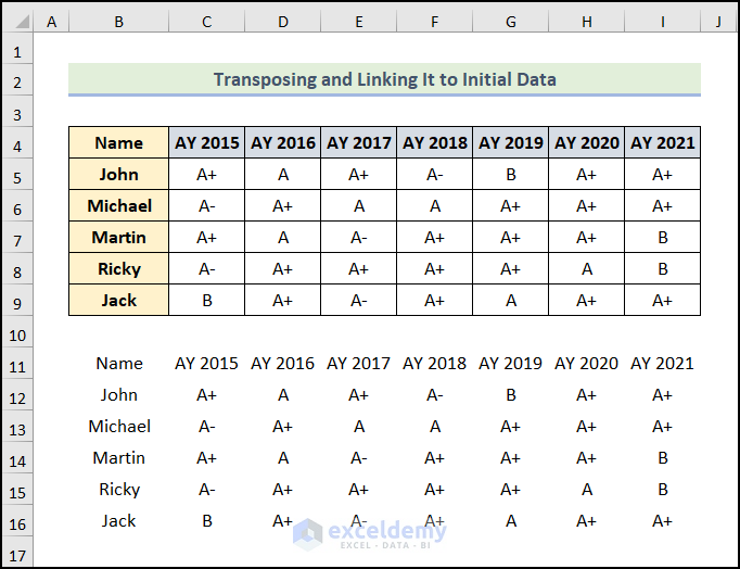
The new data set is now at the cell range of B11:I16. It’s not transposed yet. We have just linked it up with our original data set.
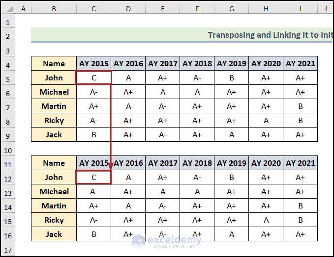
- Press CTRL + H to open the Find and Replace dialog box.
- In the Find What box, enter the equal (=) sign.
- Enter abc in the Replace with box.
- Click the Replace All button.
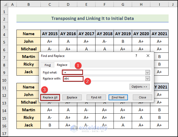
It may seem that we have lost our new data set.
![]()
- Copy the new data in the B11:I16 range.
- Follow the previous steps to paste them in the transposed form in cell K4.
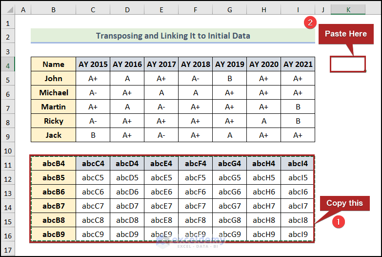
The transposed dataset is now visible in the worksheet.
![]()
- Open the Find and Replace wizard.
- Enter abc and “=” in the Find what and Replace with box.
- Click on the Replace All button.
![]()
We have generated our desired linked-up and transposed dataset.
*Note: If you change any input in the original dataset, the transposed data will also change accordingly. Look at the screenshot attached here.
Read More: How to Transpose in Excel (5 Easy Ways)
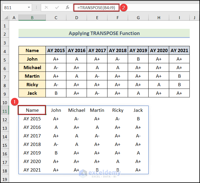
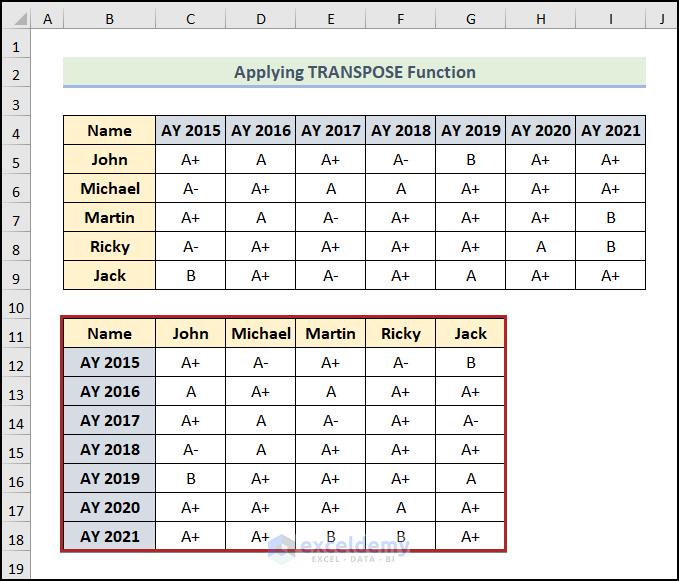
Method 3 – Applying the TRANSPOSE Function
Steps:
- Go to cell B11 and enter the following formula into the Formula Bar:
=TRANSPOSE(B4:I9)
Formula Breakdown
- The COLUMN and ROW functions return the column and row number for these cell references. As example, COLUMN(B4) returns 2, ROW(B4) returns 4. (ADDRESS(COLUMN(B4)-COLUMN($B$4)+ROW($B$4), ROW(B4)-ROW($B$4)+COLUMN($B$4)) becomes ADDRESS(4,2).
- Output → B4
- The INDIRECT function returns the value present in the stored reference. INDIRECT(ADDRESS(4,2)) becomes INDIRECT(B4).
- Output → Name
- Press the ENTER key.
Note: The TRANSPOSE function is dynamic, which means if you change anything in the original dataset, it will automatically update in the transposed output. However, the formatting cannot be transferred. So, you have to do it manually.
Read More: How to Transpose Array in Excel (3 Simple Ways)
Similar Readings
- How to Transpose Every n Rows to Columns in Excel (2 Easy Methods)
- Convert Columns to Rows in Excel Using Power Query
- How to Transpose Duplicate Rows to Columns in Excel (4 Ways)
- Transpose Multiple Columns into One Column in Excel (3 Handy Methods)
- How to Convert Multiple Columns into a Single Row in Excel (2 Ways)
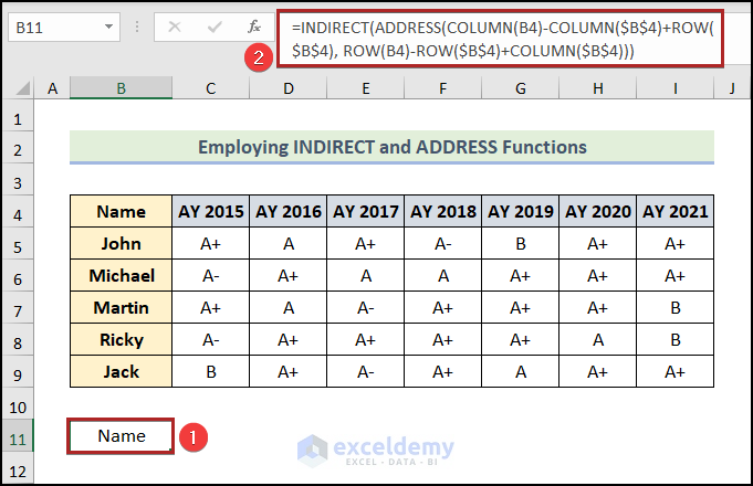
Method 4 – Employing INDIRECT and ADDRESS Functions
Steps:
- Select cell B11.
- Enter the following formula:
=INDIRECT(ADDRESS(COLUMN(B4)-COLUMN($B$4)+ROW($B$4), ROW(B4)-ROW($B$4)+COLUMN($B$4)))
- Press ENTER.
- Bring the cursor to the right-bottom corner of cell B11. It’ll look like a plus (+) sign. It’s the Fill Handle tool.
- Drag this tool up to cell G11, horizontally.
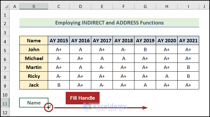
- Drag the Fill Handle tool up to cell G18, vertically.
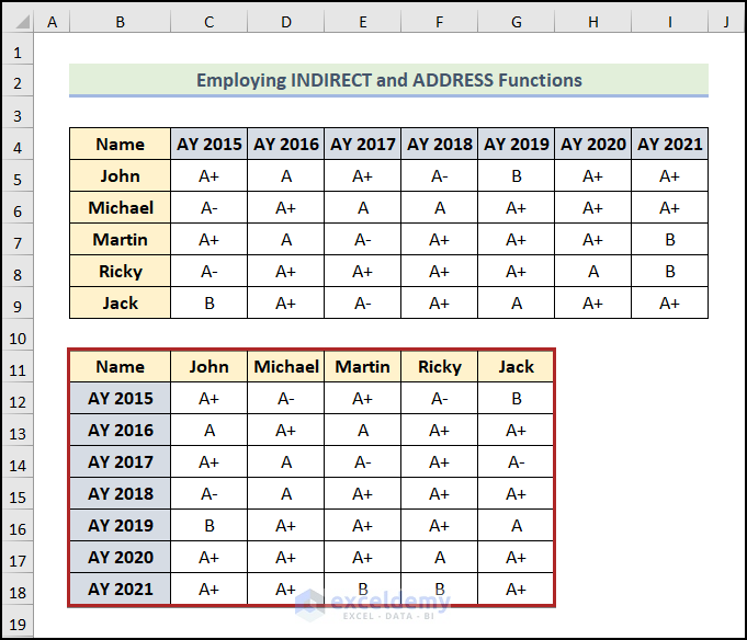
![]()
We have the transposed dataset, but it’s not formatted.
![]()
Below is what it should look like after formatting.
Read More: How to Perform Conditional Transpose in Excel (2 Easy Examples)
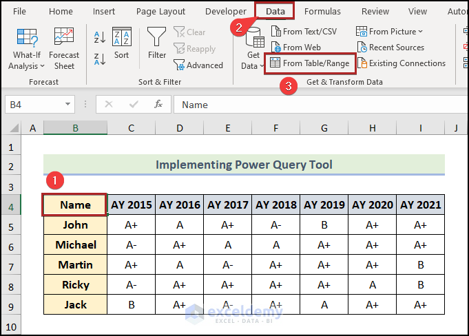
Method 5 – Implementing Power Query Tool
Steps:
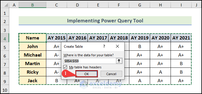
- Select any cell inside the dataset. (i.e.cell B4.)
- Go to the Data tab.
- Click on From Table/Range on the Get & Transform Data group.
The Create Table dialog box opens.
- Click OK.
The Power Query Editor window will open.
- Go to the Transform tab.
- Select Use Headers as First Row.
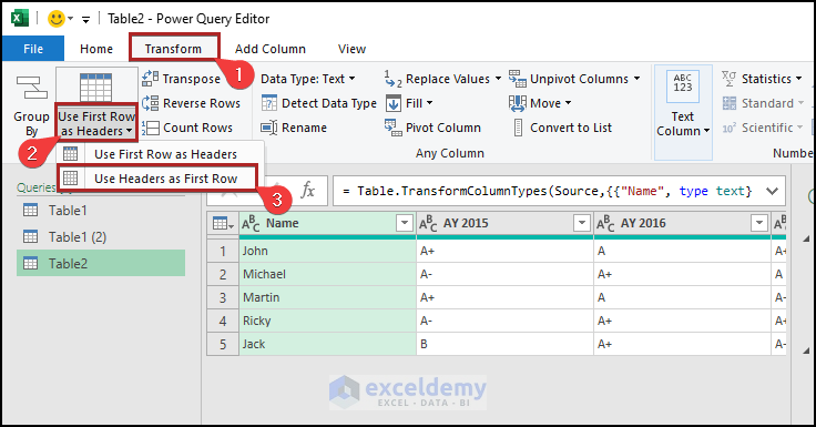
- Click Transpose.
![]()
- Go to the Transform tab and select Use First Row as Headers.
![]()
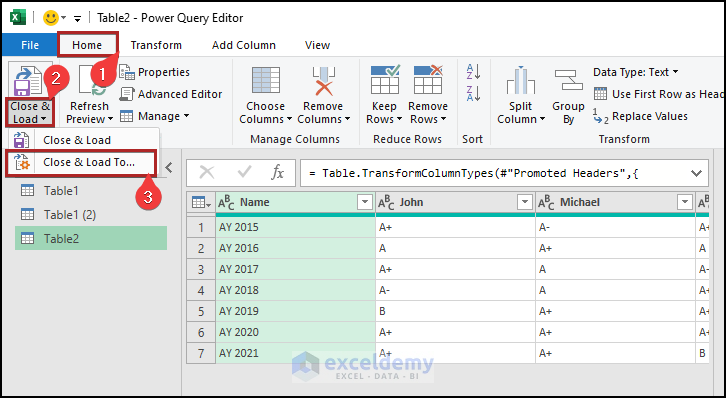
- Go to the Home tab.
- Click on the Close & Load drop-down icon.
- Select Cose & Load.
The Import Data wizard will open up.
- Select the Existing worksheet as Where do you want to put the data?
- Enter the cell reference of B11 in the box.
- Click OK.
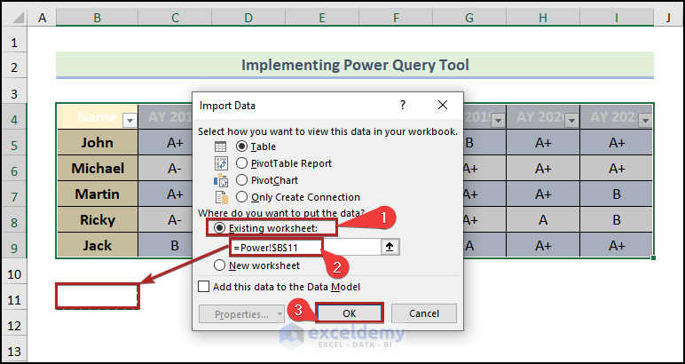
The Power Query Editor dialog box will be closed, and the transposed data will be loaded into the “Power Query“ worksheet.
Read More: Excel Power Query: Transpose Rows to Columns (Step-by-Step Guide)
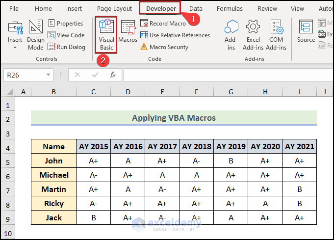
Method 6 – Applying VBA Macros
Steps:
- Go to the Developer tab.
- Click on Visual Basic in the Code group.
The Microsoft Visual Basic for Applications window appears.
- Go to the Insert tab.
- Select Module from the options.
![]()
Excel will insert a code module.
- Paste the following code into the module:
Option Explicit
Sub Rows_to_Columns()
    Dim Sr_Rng As Range
    Dim Dst_Rng As Range
    Set Sr_Rng = Application.InputBox(Prompt:="Mark the range to flip", Title:="ExcelDemy: Transpose Tool", Type:=8)
    Set Dst_Rng = Application.InputBox(Prompt:="Mark the cell where you want to place the transposed range", Title:="ExcelDemy: Transpose Tool", Type:=8)
    Sr_Rng.Copy
    Dst_Rng.Select
    Selection.PasteSpecial Paste:=xlPasteAll, Operation:=xlNone, SkipBlanks:=False, Transpose:=True
    Application.CutCopyMode = False
End Sub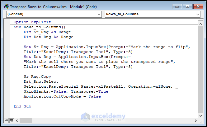
Code Breakdown
- We mentioned the sub-procedure name and declared the variables.
- We inserted two InputBoxes. The values received in the InputBox will be taken by the variable.
- We applied the Copy method to copy the range and paste it into the transposed form in the range of the second variable.
- We ended the sub-procedure with End Sub.
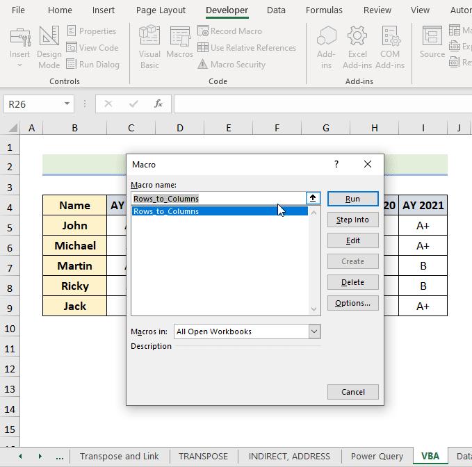
- Save the file as Macro-Enabled Workbook and return to the VBA worksheet. Follow the GIF to understand the next procedures.
We’ve converted the rows into columns using the VBA macros.
Read More: How to Transpose Rows to Columns Using Excel VBA (4 Ideal Examples)
Method 7 – Using Criteria in Excel
Steps:
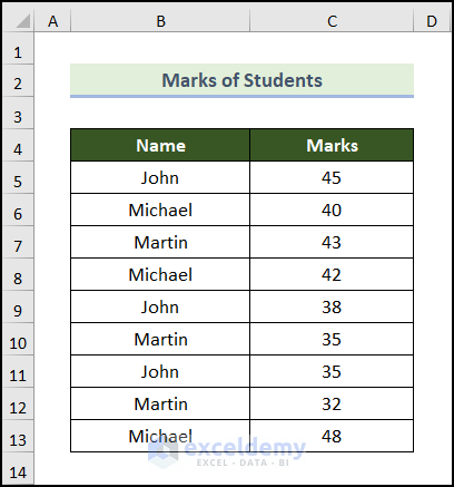
Below is a dataset with the Marks of Students. It contains the Name and corresponding Marks in columns B and C.
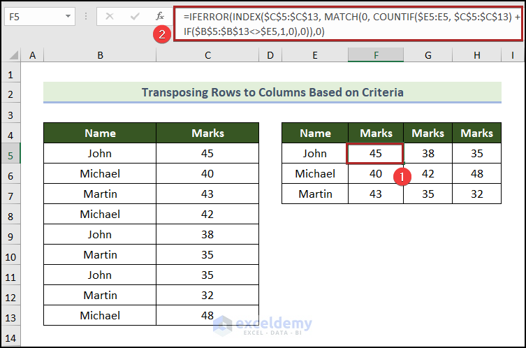
- Create a new table in the E4:H7 with headings Name, and Marks.
![]()
- Go to cell E5 and insert the following formula:
=INDEX($B$5:$B$13, MATCH(0, COUNTIF($E$4:$E4, $B$5:$B$13), 0))
Formula Breakdown
- COUNTIF($E$4:$E4, $B$5:$B$13) returns an array of 0 because it couldn’t find the text string Name in the B5:B13
- Then, MATCH(0, COUNTIF($E$4:$E4, $B$5:$B$13), 0) becomes MATCH(0, {0,0,0,0,0,0,0,0,0}, 0).
- Output → 1
- INDEX($B$5:$B$13, MATCH(0, COUNTIF($E$4:$E4, $B$5:$B$13), 0)) becomes INDEX($B$5:$B$13, 1).
- Output → John
- Press ENTER.
![]()
The formula used to get the marks is the following:
=IFERROR(INDEX($C$5:$C$13, MATCH(0, COUNTIF($E5:E5, $C$5:$C$13) + IF($B$5:$B$13<>$E5,1,0),0)),0)
You can follow the article How to Transpose Rows to Columns Based on Criteria in Excel on our website.
Practice Section
![]()
Download the Practice Workbook
You may download the following Excel workbook.
Related Articles
- How to Transpose Columns to Rows In Excel (6 Methods)
- How to Convert Columns to Rows in Excel Based On Cell Value
- VBA to Transpose Multiple Columns into Rows in Excel (2 Methods)
- How to Swap Rows in Excel (2 Methods)
- Convert Columns to Rows in Excel (2 Methods)
- Excel Transpose Formulas Without Changing References (4 Easy Ways)

