25 VBA Macro Example for Enhanced Productivity

How to Launch and Insert Code in the Visual Basic Editor in Excel

The Developer tab contains the VBA applications including creating and recording macros, Excel Add-ins, Forms controls, importing and exporting XML data, etc.
By default, the Developer tab is hidden.

• You’ll need to display the Developer tab first.
• Once enabled, go to the Developer tab, then click on the Visual Basic button in the Code group.

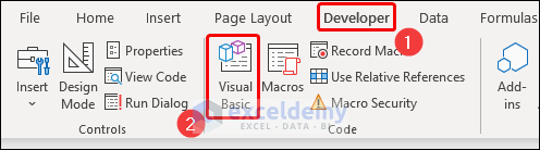
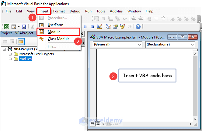
This launches the Microsoft Visual Basic for Applications window.

• Click the Insert tab and choose Module from the list. We get a small Module window to insert the VBA code.

How to Run Macro in Excel?

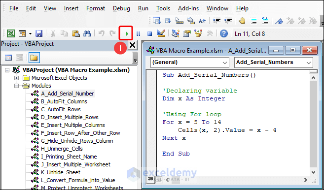
• After entering the code script, click the green-colored play button to Run the code. You can also press F5 on the keyboard.

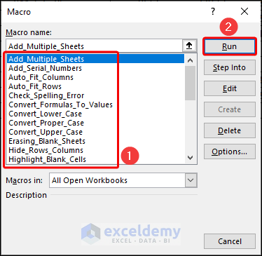
Another way is to execute it from the Macro dialog box:

• Click on the Developer tab and select Macros in the Code group of commands on the ribbon.

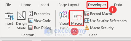
• A Macro dialog box will pop up. You can see multiple Macros available which were created for the workbook.
• Select one and click on the Run button.

25 Useful VBA Macro Example in Excel

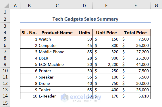
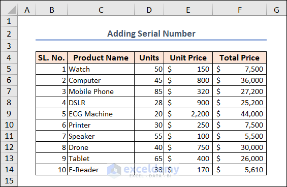
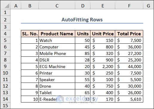
We will use the following dataset to perform the exercises. This is the “Tech gadgets Sales Summary” of a particular shop. The dataset includes the “SL. No”, “Product Name”, “Units”, “Unit Price”, and “Total Price” in columns B, C, D, E, and F, respectively.

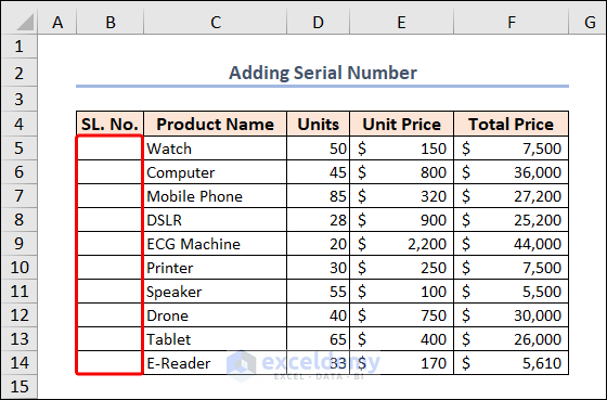
Example 1 – Adding a Serial Number

We have a blank Column B. We’ll fill up these cells with the serial number.

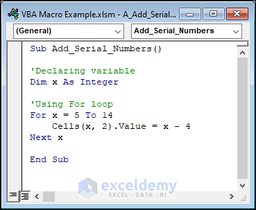
Use the below code to complete this task.

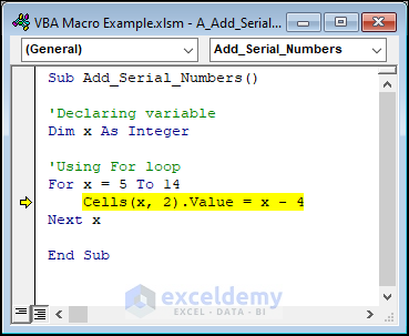
Sub Add_Serial_Numbers()
'Declaring variable
Dim x As Integer
'Using For loop
For x = 5 To 14
    Cells(x, 2).Value = x - 4
Next x
End Sub

The objective of this macro is to adjoin serial numbers in Column B of an Excel sheet. The macro utilizes a loop to cycle over the rows from Row 5 to Row 14 (where x denotes the row number), deducting 4 from each row’s row number and assigning the result to the cell in Column B that corresponds to that row.

After running this macro, it will add serial numbers in the spreadsheet from 1 to 10 in the B5:B14 range.

Read More: Types of VBA Macros in Excel

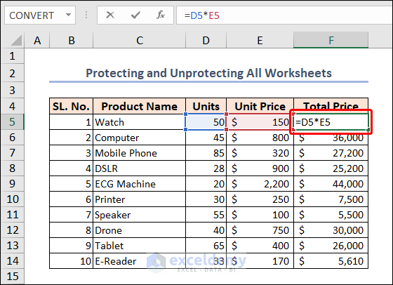
Example 2 – Converting All Formulas into Values

You will find all the formulas in Column F.

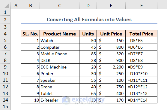
You can use the following code.

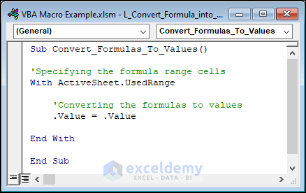
Sub Convert_Formulas_To_Values()
'Specifying the formula range cells
With ActiveSheet.UsedRange
    'Converting the formulas to values
    .Value = .Value
End With
End Sub

The code converts all the formulas in the active sheet to their resulting values.

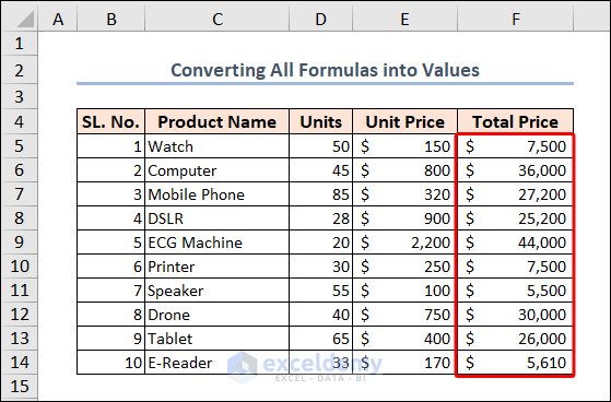
This can be useful when you want to preserve the results of a calculation or analysis, but no longer need the original formulas.
Note: This action cannot be undone, so it’s a good idea to make a backup copy of your worksheet before running this macro.

Read More: Excel Macro Shortcut Key

Example 3 – Auto-Fitting Columns and Rows

The column width in some cells isn’t high enough to display values.

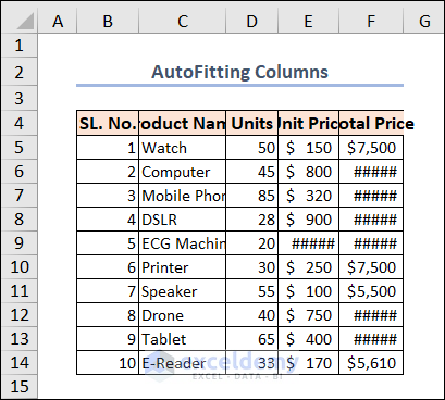
The same thing goes for improper row heights.

Use the following code to Auto-Fit columns.

Sub Auto_Fit_Columns()
Cells.Select
'Auto fit the entire column
Cells.EntireColumn.AutoFit
End Sub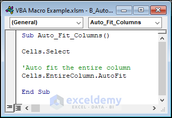

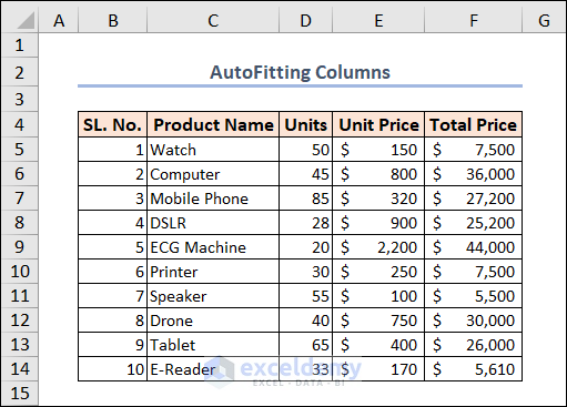
All columns get auto-fitted in this particular sheet.

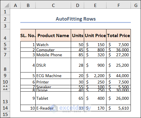
Auto-fitting rows uses this code:

Sub Auto_Fit_Rows()
Cells.Select
'Auto fit the entire row
Cells.EntireRow.AutoFit
End Sub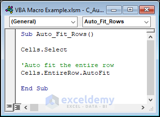

Here’s the result.

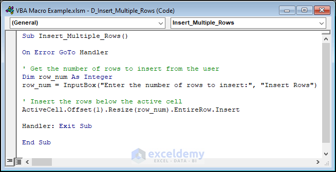
Example 4 – Inserting Multiple Rows and Columns

Sub Insert_Multiple_Rows()
On Error GoTo Handler
' Get the number of rows to insert from the user
Dim row_num As Integer
row_num = InputBox("Enter the number of rows to insert:", "Insert Rows")
' Insert the rows below the active cell
ActiveCell.Offset(1).Resize(row_num).EntireRow.Insert
Handler: Exit Sub
End Sub

ActiveCell.Offset(1).Resize(row_num).EntireRow.Insert in this VBA code inserts a certain number of rows beneath the active (selected) cell in an Excel worksheet. Here’s how this line of code works:

• ActiveCell refers to the presently selected cell in the worksheet.
• Offset(1) moves the active cell down one row. This is so that the new rows can be inserted below the current cell rather than above it.
• Resize(row_num) changes the selection’s size to match the number of rows indicated by the row_num variable, which corresponds to the number of rows the user supplied in the input box earlier in the code.
• EntireRow selects the full resized row or rows.
• Last but not least, Insert adds a new row or rows to the worksheet beneath the active cell.

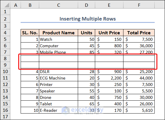
• Let’s say we want to add rows below the row of SL. No. 3. We selected cell B7 and then run the code.
• When the code runs, an input box pops up to get the number of rows to be inserted below the selected cell. Input your preferred number to get new rows of this count. We inserted 2.
• Click OK.

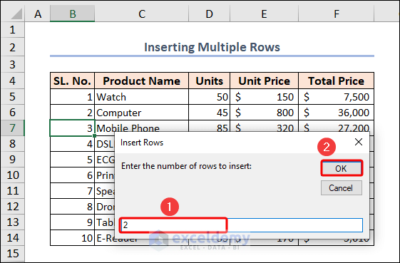
The code adds two rows beneath Row 7.

For inserting multiple columns in our dataset, we’ll use this code:

Sub Insert_Multiple_Columns()
' Get the number of columns to insert from the user
Dim col_num As Integer
col_num = InputBox("Enter the number of columns to insert:", "Insert Columns")
' Insert the columns to the right of the active cell
ActiveCell.Offset(0, 1).Resize(, col_num).EntireColumn.Insert
End Sub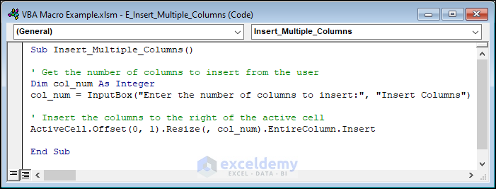

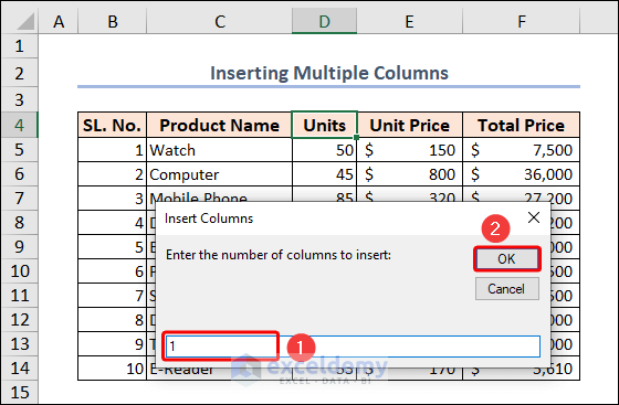
• Before initiating the code, we selected cell D4, as we want to insert columns after Column D.
• Run the code.
• Enter your desired integer number and click OK.

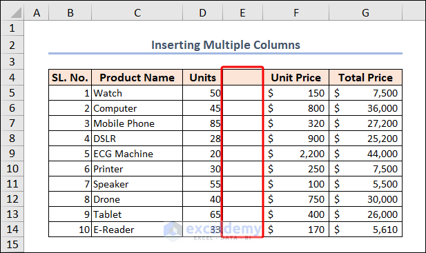
The following image is resemblance to the final output.

Example 5 – Inserting a Row After Every Other Row

Copy and paste this code into your code module.

Sub Insert_Row_After_Every_Other_Row()
'Declaring Variables
Dim Xrng As Range
Dim row_count As Integer
Dim j As Integer
Set Xrng = Selection
'Counting rows
row_count = Xrng.EntireRow.Count
'using For loop
For j = 1 To row_count
    'Inserting row after every other row
    ActiveCell.EntireRow.Insert
    ActiveCell.Offset(2, 0).Select
Next j
End Sub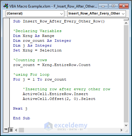

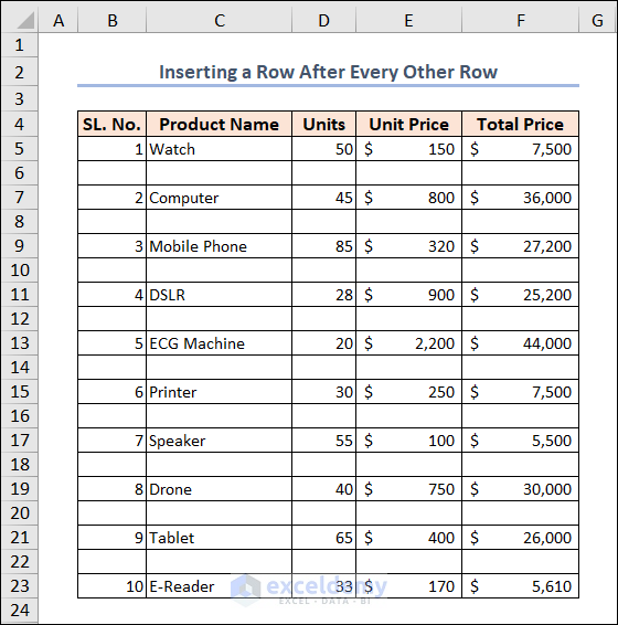
We selected the B6:F14 range in our dataset, then ran the code.
The result is as follows.

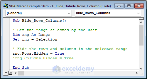
Example 6 – Hiding and Unhiding Rows and Columns

For hiding rows, the code is the following:

Sub Hide_Rows_Columns()
' Get the range selected by the user
Dim rng As Range
Set rng = Selection
' Hide the rows and columns in the selected range
rng.Rows.Hidden = True
'rng.Columns.Hidden = True
End Sub

We have kept a line of code in the comment form, because we’ll use this part to hide columns.

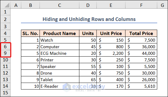
• Select the row or rows which you want to hide and run the code.

We can hide the columns with the modified code:

Sub Hide_Rows_Columns()
' Get the range selected by the user
Dim rng As Range
Set rng = Selection
' Hide the rows and columns in the selected range
'rng.Rows.Hidden = True
rng.Columns.Hidden = True
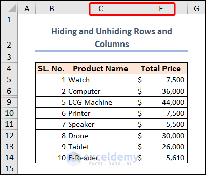
End Sub

You can see columns D and E aren’t visible also.

• We’ll unhide these hidden rows and columns with this code:

Sub Unhide_Rows_Columns()
'Unhide columns
Columns.EntireColumn.Hidden = False
'Unhide rows
Rows.EntireRow.Hidden = False
End Sub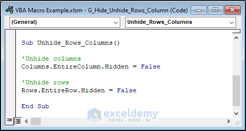

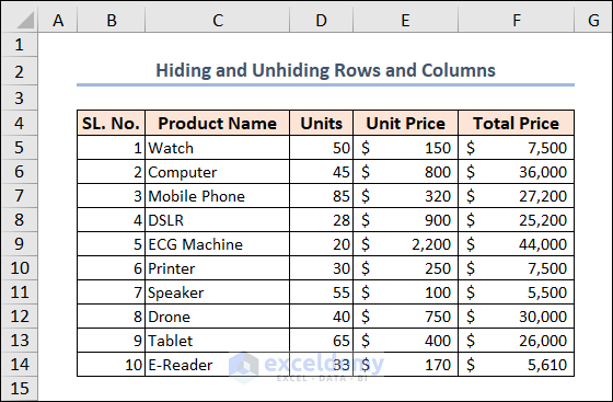
The resulting output is as follows.

Example 7 – Finding the Last Used Row in an Excel Worksheet

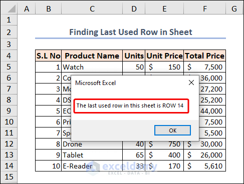
Row 14 is the last used row in our case.

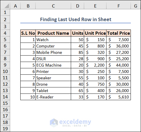
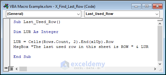
Here’s the code that finds that row.

Sub Last_Used_Row()
Dim LUR As Integer
LUR = Cells(Rows.Count, 2).End(xlUp).Row
MsgBox "The last used row in this sheet is ROW " & LUR
End Sub

We used the Cells function to select the cell in the last row of Column B (Rows.Count returns the total number of rows in the worksheet, and End(xlUp) moves up from the bottom of the sheet to the last cell with a value).

The Row property returns the row number of the selected cell.

You get a message box with the message containing the last used row number after running the code.

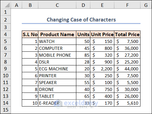
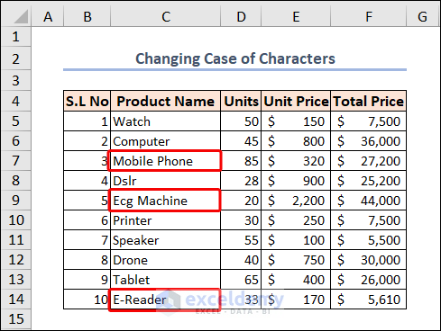
Example 8 – Changing the Case of Characters

We’ll take the column Product Name, convert all values to upper case, then to proper case, then to lowercase.

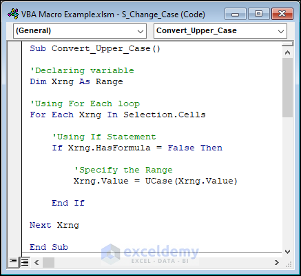
This macro code works converts all the text values to uppercase.

Sub Convert_Upper_Case()
'Declaring variable
Dim Xrng As Range
'Using For Each loop
For Each Xrng In Selection.Cells
    'Using If Statement
    If Xrng.HasFormula = False Then
        'Specify the Range
        Xrng.Value = UCase(Xrng.Value)
    End If
Next Xrng
End Sub

We used Xrng.HasFormula = False in the If statement to omit values that got formula. If the value isn’t the output of a formula, then we changed its case only. We used the UCase function to achieve the main part.

Select the range before executing the code.

In the proper case, the first letter of each word gets written in capital letters, and the remaining in small letters. Here’s the working code to do this:

Sub Convert_Proper_Case()
'Declaring variable
Dim rng As Range
'Using For Each loop
For Each rng In Selection
    'Reading the worksheet text range cells
    If WorksheetFunction.IsText(rng) Then
        'Converting all the selected range to proper case
        rng.Value = WorksheetFunction.Proper(rng.Value)
    End If
Next rng
End Sub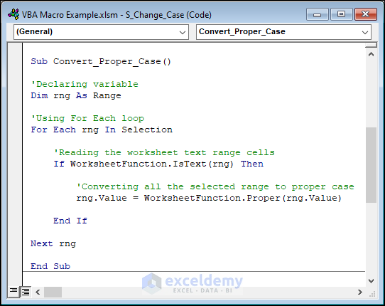

Select the range before initiating the code.

We’ll convert all the texts in Column C to lowercase characters. Use this code to do this:

Sub Convert_Lower_Case()
'Declaring variable
Dim Xrng As Range
'Using For Each loop
For Each Xrng In Selection.Cells
     'Using If Statement
    If Xrng.HasFormula = False Then
       'Specify the Range
        Xrng.Value = LCase(Xrng.Value)
   End If
Next Xrng
End Sub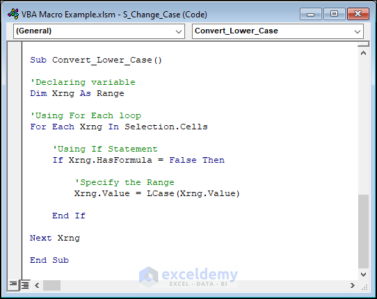

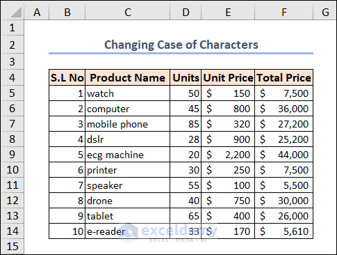
Select the range before you run the code and the final results are displayed in the graphic below, which only has lowercase text.

Example 9 – Highlighting Multiple Blank Cells

There are multiple blank cells in our worksheet.

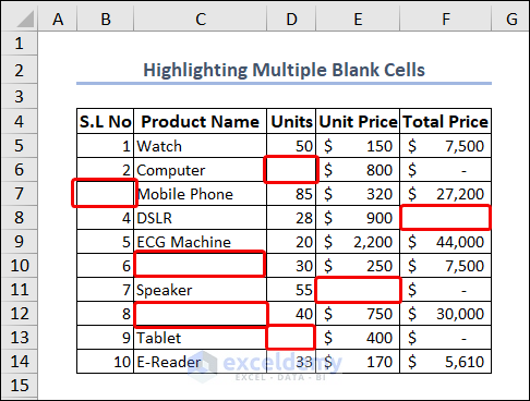
The VBA code to highlight them is:

Sub Highlight_Blank_Cells()
'Declaring variable
Dim MyData As Range
Set MyData = Selection
'Highligting the selected data range with color
MyData.Cells.SpecialCells(xlCellTypeBlanks).Interior.Color = vbGreen
End Sub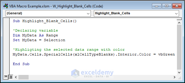

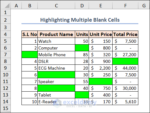
Select the data range and run the macro.

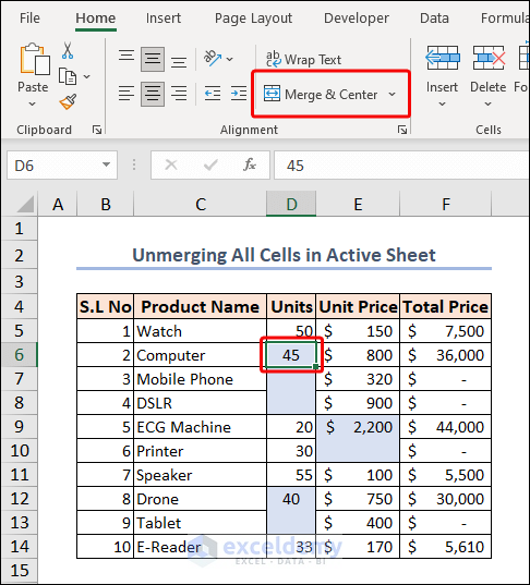
Example 10 – Unmerging All Cells in the Active Sheet

In the following image, there are some merged cells highlighted with a different background fill color.

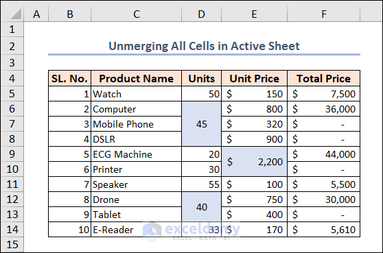
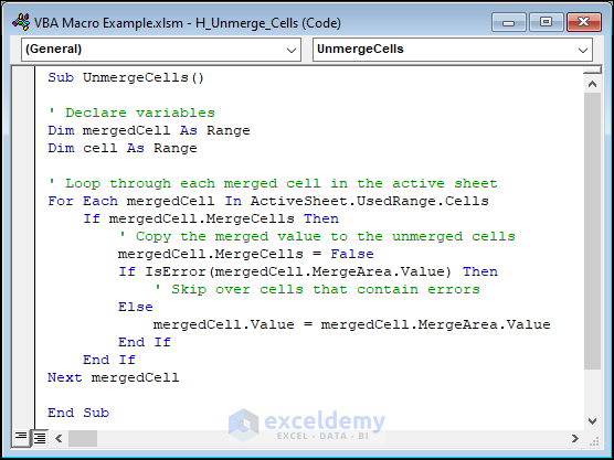
Let’s unmerge those cells. Use the following code to do this.

Sub UnmergeCells()
' Declare variables
|Dim mergedCell As Range
Dim cell As Range
' Loop through each merged cell in the active sheet
For Each mergedCell In ActiveSheet.UsedRange.Cells
    If mergedCell.MergeCells Then
        ' Copy the merged value to the unmerged cells
        mergedCell.MergeCells = False
        If IsError(mergedCell.MergeArea.Value) Then
            ' Skip over cells that contain errors
        Else
            mergedCell.Value = mergedCell.MergeArea.Value
        End If
    End If
Next mergedCell
End Sub

The values in those cells are not center aligned. They get top-aligned as they are not merged anymore. If you select one of them, you can see the Merge & Center command isn’t highlighted as they got unmerged now.

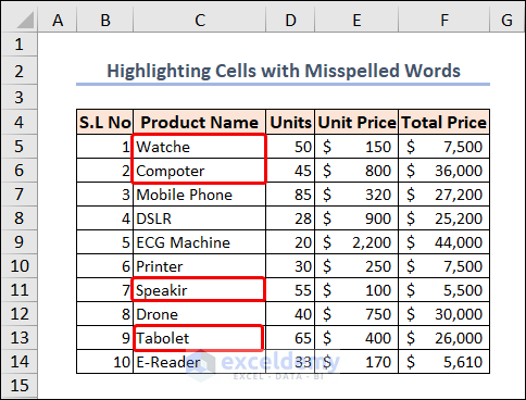
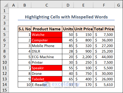
Example 11 – Highlighting Cells with Misspelled Words in Excel

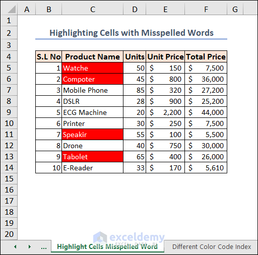
Spell checking is not available in Excel like it is in Word or PowerPoint. We can see there are some misspelled words in our dataset.

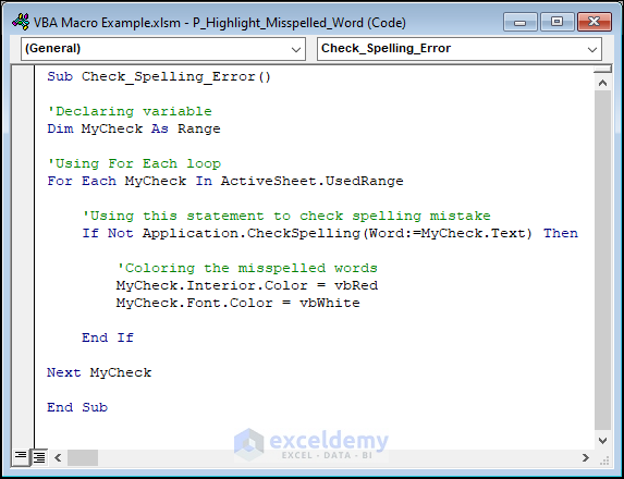
You can use this code to highlight every cell that contains a spelling error.

Sub Check_Spelling_Error()
'Declaring variable
Dim MyCheck As Range
'Using For Each loop
For Each MyCheck In ActiveSheet.UsedRange
     'Using this statement to check spelling mistake
    If Not Application.CheckSpelling(Word:=MyCheck.Text) Then
        'Coloring the misspelled words
        MyCheck.Interior.Color = vbRed
        MyCheck.Font.Color = vbWhite
    End If
Next MyCheck
End Sub

In this code, “If Not Application.CheckSpelling(Word:=MyCheck.Text) Then”, this line uses the Application.CheckSpelling method to check for spelling errors in the text of the current cell (MyCheck.Text). If the CheckSpelling method returns False, which indicates a spelling error, then the code inside the If statement will be executed.

MyCheck.Interior.Color = vbRed
MyCheck.Font.Color = vbWhite

This code sets the interior color of the current cell to red (vbRed) and the font color to white (vbWhite) to highlight the misspelled word.

Each highlighted misspelled word you have will be highlighted.

Example 12 – Printing the Sheet Name

The active sheet will receive all the sheet names by this macro code.

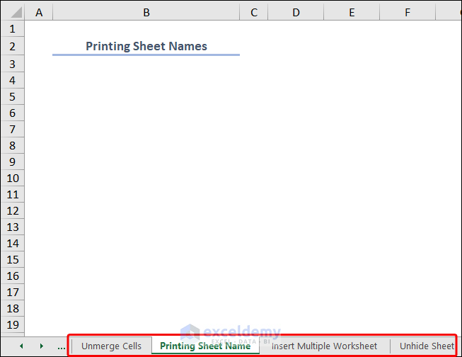
We’ll fill the sheet names in Column B with this code:

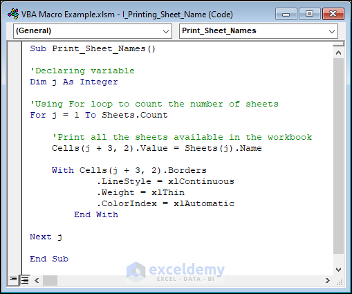
Sub Print_Sheet_Names()
'Declaring variable
Dim j As Integer
'Using For loop to count the number of sheets
For j = 1 To Sheets.Count
     'Print all the sheets available in the workbook
    Cells(j + 3, 2).Value = Sheets(j).Name
    With Cells(j + 3, 2).Borders
            .LineStyle = xlContinuous
           .Weight = xlThin
            .ColorIndex = xlAutomatic
        End With
Next j
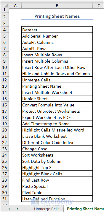
End Sub

This VBA code copies the names of all the sheets available in the workbook. It uses a For loop to iterate through each sheet and prints its name in a specific cell using the Cells method. Additionally, it also applies a border to the cell containing the sheet name.

Here’s the result.

Example 13 – Sorting Worksheets Alphabetically

We have several unsorted sheets.

This macro code organizes them from A to Z.

Sub Sort_Worksheets_Alphabetically()
'Fast the code running time
Application.ScreenUpdating = False
'Declaring variables
Dim MySheetCount As Integer, x As Integer, y As Integer
MySheetCount = Sheets.Count
'Using nested For loop to sort the worksheets alphabetically
For x = 1 To MySheetCount - 1
    For y = x + 1 To MySheetCount
        If UCase(Sheets(y).Name) < UCase(Sheets(x).Name) Then
            Sheets(y).Move before:=Sheets(x)
        End If
    Next y
Next x
Application.ScreenUpdating = True
End Sub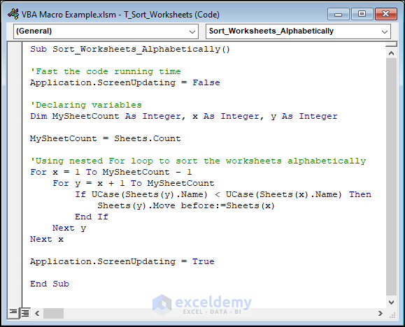

After running the above macro, you will all the sheet names in order alphabetically.

Example 14 – Inserting Multiple Worksheets in an Excel Workbook

This code inserts multiple worksheets.

Sub Add_Multiple_Sheets()
'Declaring variable
Dim SheetsNumber As Integer
'Put the number of sheets
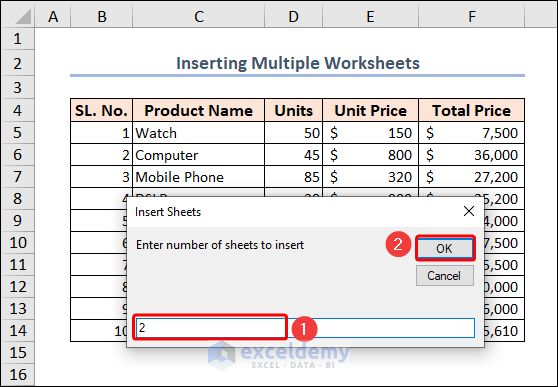
SheetsNumber = InputBox("Enter number of sheets to insert", "Insert Sheets")
'Adding the additional sheets after the current active sheet
Sheets.Add After:=ActiveSheet, Count:=SheetsNumber
End Sub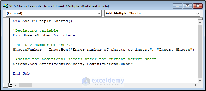

When you run the code, an input box will open to get the number of worksheets to insert after the active sheet. In this case, we wrote 2 and clicked OK.

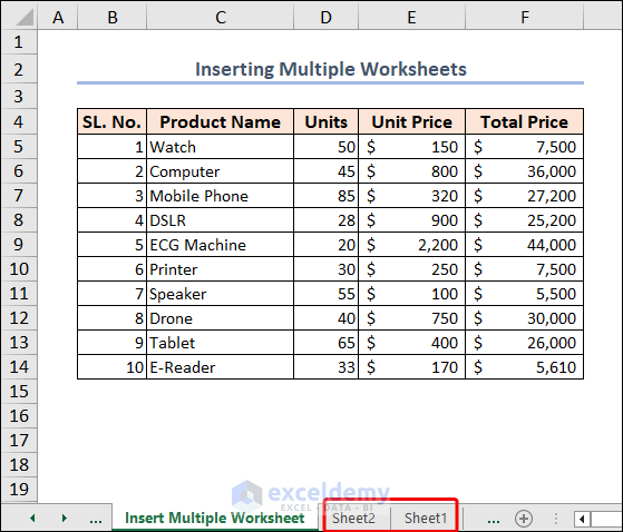
The code added two blank sheets after the operating sheet.

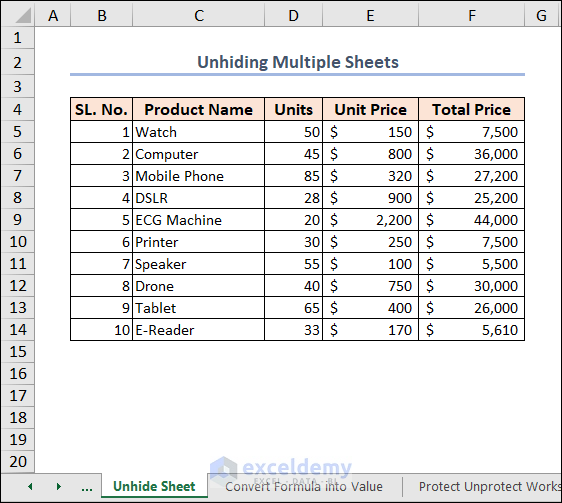
Example 15 – Unhiding Multiple Sheets

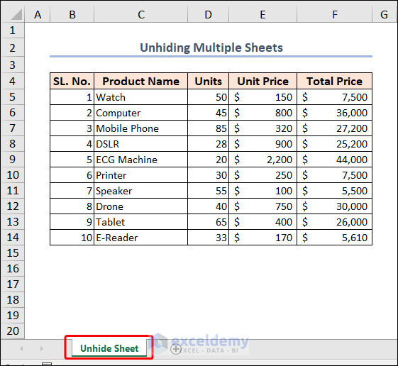
In the image below, there is one sheet visible in the workbook. All others are hidden.

This code will display every worksheet in the workbook.

Sub Unhide_Multiple_Sheets()
'Declaring variable
Dim hidden_sheet As Worksheet
'Using For Each loop
For Each hidden_sheet In ActiveWorkbook.Worksheets
     'All the sheets will be visible
     hidden_sheet.Visible = xlSheetVisible
Next hidden_sheet
End Sub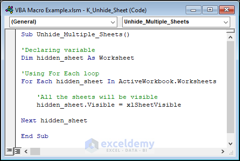

After executing the code, all other sheets are visible/unhidden again.

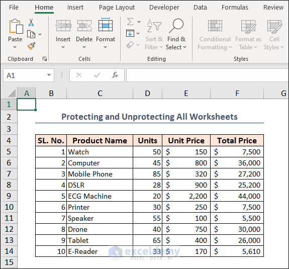
Example 16 – Protecting and Unprotecting All Worksheets

The VBA code to protect your worksheets is:

Sub Protect_Multiple_Sheets()
'Declaring variable
Dim MySheet As Worksheet
'Using For loop
For Each MySheet In Worksheets    
    'Protecting multiple sheets
    MySheet.Protect
Next MySheet
End Sub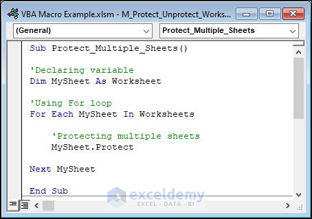

Most of the commands and features on the ribbon get greyed out. That means they are not available now. You cannot use them to edit, or change your worksheet.

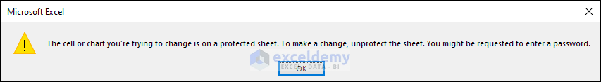
If you tried to enter any value or change any value, Excel will show a message box like the following.

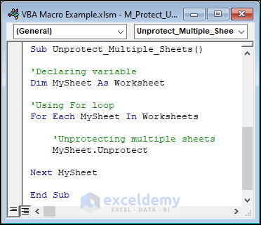
If we want to unprotect sheets again, just use the code below.

Sub Unprotect_Multiple_Sheets()
'Declaring variable
Dim MySheet As Worksheet
'Using For loop
For Each MySheet In Worksheets
    'Unprotecting multiple sheets
    MySheet.Unprotect
Next MySheet
End Sub

We just changed the . Protect method to the .Unprotect method.

We can edit anything on the worksheet.

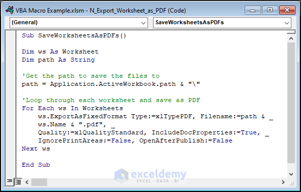
Example 17 – Exporting Individual Worksheets as PDF Files

Here’s the VBA code that exports individual worksheets in a workbook as PDF files.

Sub SaveWorksheetsAsPDFs()
Dim ws As Worksheet
Dim path As String
'Get the path to save the files to
path = Application.ActiveWorkbook.path & "\"
'Loop through each worksheet and save as PDF
For Each ws In Worksheets
    ws.ExportAsFixedFormat Type:=xlTypePDF, Filename:=path & _
    ws.Name & ".pdf", _
    Quality:=xlQualityStandard, IncludeDocProperties:=True, _
    IgnorePrintAreas:=False, OpenAfterPublish:=False
Next ws
End Sub

The current worksheet is saved as a PDF file inside the loop using the Worksheet object’s ExportAsFixedFormat method. There are numerous parameters that must be given for the method:

• Type: This describes the file format; for PDF files, it is “xlTypePDF” in this example.
• Filename: This gives the name and location of the finished PDF file. The name of the worksheet and the “.pdf” extension are combined with the path variable to form the whole filename.
• Quality: The PDF quality option, in this case “xlQualityStandard,” is specified by this.
• IncludeDocProperties: In this code, it is set to True, indicating that document properties should be included in the output file.
• IgnorePrintAreas: This specifies whether to ignore print areas and print the entire worksheet, which is set to False in this code.
• OpenAfterPublish: This specifies whether to open the saved PDF file after it’s created, which is set to False in this code.

Each worksheet in the active workbook is saved as a separate PDF file in the designated file location when this code is executed.

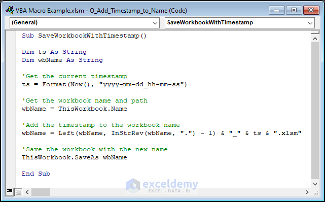
Example 18 – Adding a Timestamp to the Workbook Name While Saving

This code will save a copy of the main workbook with a timestamp in its name.

Sub SaveWorkbook_With_Timestamp()
Dim ts As String
Dim wbName As String
'Get the current timestamp
ts = Format(Now(), "yyyy-mm-dd_hh-mm-ss")
'Get the workbook name and path
wbName = ThisWorkbook.Name
'Add the timestamp to the workbook name
wbName = Left(wbName, InStrRev(wbName, ".") - 1) & "_" & ts & ".xlsm"
'Save the workbook with the new name
ThisWorkbook.SaveAs wbName
End Sub

Here, “wbName = Left(wbName, InStrRev(wbName, “.”) – 1) & “_” & ts & “.xlsm”
This line uses the Left() function to get all characters of the wbName variable from the beginning to the position of the last dot (.) minus 1, which removes the file extension. Then, it appends an underscore, the timestamp (ts variable), and the file extension “.xlsm” to the wbName variable, creating a new name with the timestamp appended.

Note: This will save the workbook as a macro-enabled workbook (.xlsm) since the original workbook likely has VBA code in it. If the original workbook is not macro-enabled, you may need to change the file format to the appropriate type (e.g., .xlsx) in the SaveAs method. And that’s it! The workbook will be saved with the timestamp appended to its name, allowing you to create unique copies of the workbook with different timestamps for version control or tracking purposes.
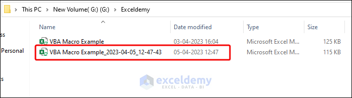
You can see the output. A new copy of this file is saved with the perfect timestamp in its name and also in the same folder of the source workbook.

Example 19 – Erasing Blank Worksheets

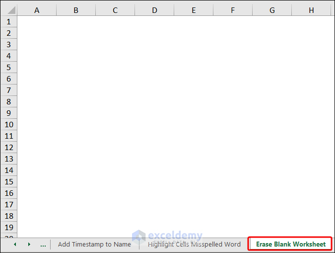
We have a blank worksheet named “Erase Blank Worksheet” in our workbook. It’s just beside the worksheet “Highlight Cells Misspelled Word”.

This macro will erase all the blank worksheets from the workbook we are using.

Sub Erasing_Blank_Sheets()
'Declaring variable
Dim MySheet As Worksheet
Application.DisplayAlerts = False
Application.ScreenUpdating = False
'Using For Each loop
For Each MySheet In ActiveWorkbook.Worksheets
    'using this statement to Count blank sheets
    If WorksheetFunction.CountA(MySheet.UsedRange) = 0 Then
        'Deleting blank sheets
        MySheet.Delete
    End If
Next MySheet
Application.DisplayAlerts = True
Application.ScreenUpdating = True
End Sub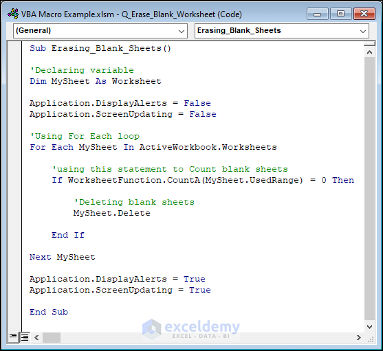

Here’s the result.

Example 20 – Inserting Different Colors Based on the Color Index

We will insert numbers from 1 to 10 and their respective color index in the next column. We have the worksheet in this state now.

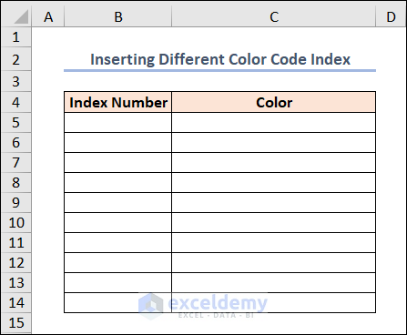
In Column B, we’ll enter numbers and in the right next column, we’ll insert their respective color index.

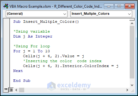
The following VBA code will fill the cells based on the color code.

Sub Insert_Multple_Colors()
'Using variable
Dim j As Integer
'Using For loop
For j = 1 To 10
    Cells(j + 4, 2).Value = j
    'Inserting the color  code index
    Cells(j + 4, 3).Interior.ColorIndex = j
Next
End Sub

Here’s the output.

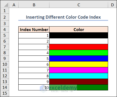
Excel has 56 built-in colors with corresponding index numbers, and this code uses the index number to set the background color of the cell.

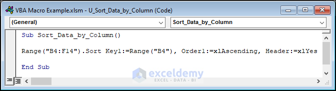
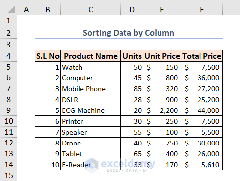
Example 21 – Sorting Data by Column

In the following image, we can see that our data isn’t arranged properly. Their serial numbers aren’t arranged properly but rather in a random serial.

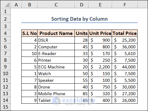
We’ll sort this dataset based on the serial numbers in Column B. The code is given below.

Sub Sort_Data_by_Column()
Range("B4:F14").Sort Key1:=Range("B4"), Order1:=xlAscending, Header:=xlYes
End Sub

The Sort method takes three arguments:

• Key1: This specifies the column by which the data is sorted. In this case, the sort key is set to the range “B4“, which means that the data is sorted based on the values in Column B.
• Order1: This specifies the sort order. In this case, the sort order is set to “xlAscending“, which means that the data is sorted in ascending order (e.g 0, 1, 2, 3,…, 10).
• Header: This specifies whether the range has a header row that should not be sorted. In this case, the header is set to “xlYes“, which means that the first row of the range (“B4:F4“) is treated as a header row and is not sorted with the data.

Here’s the result.

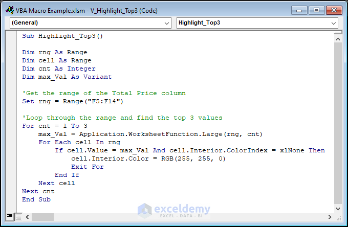
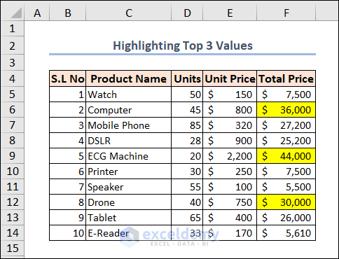
Example 22 – Highlighting Top 3 Values

Use this code:

Sub Highlight_Top3()
Dim rng As Range
Dim cell As Range
Dim cnt As Integer
Dim max_Val As Variant
'Get the range of the Total Price column
Set rng = Range("F5:F14")
'Loop through the range and find the top 3 values
For cnt = 1 To 3
    max_Val = Application.WorksheetFunction.Large(rng, cnt)
    For Each cell In rng
        If cell.Value = max_Val And cell.Interior.ColorIndex = xlNone Then
            cell.Interior.Color = RGB(255, 255, 0)
            Exit For
        End If
    Next cell
Next cnt
End Sub

You can see the result here.

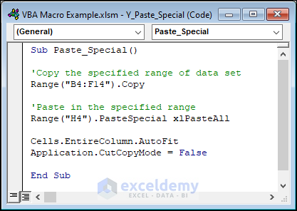
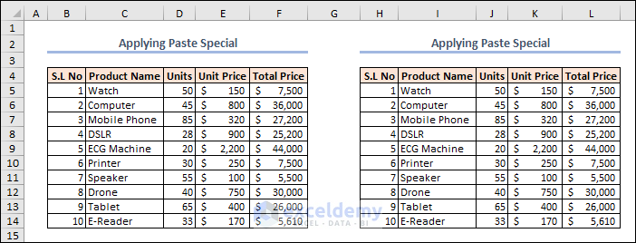
Example 23 – Applying Paste Special

The code is:

Sub Paste_Special()
'Copy the specified range of data set
Range("B4:F14").Copy
'Paste in the specified range
Range("H4").PasteSpecial xlPasteAll
Cells.EntireColumn.AutoFit
Application.CutCopyMode = False
End Sub

This code copies the B4:F14 range and pastes it in the H4 range using the Paste Special method.

Here’s the result.

Example 24 – Refreshing Pivot Tables in the Workbook

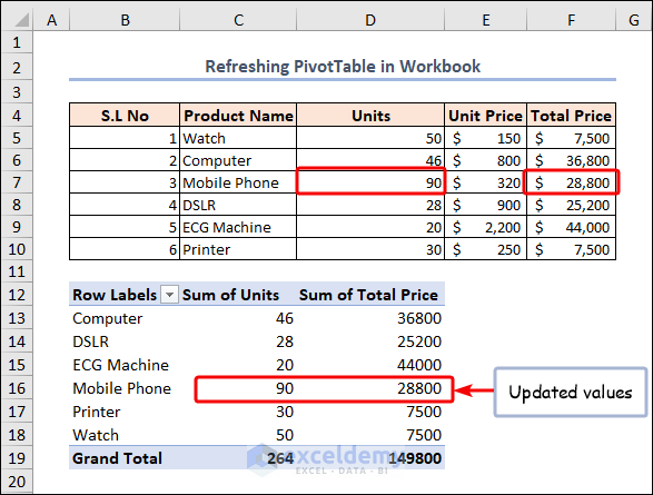
We have created a PivotTable from the data in the B4:F10 range. If you don’t know how to create a PivotTable in Excel, you can follow the linked article.

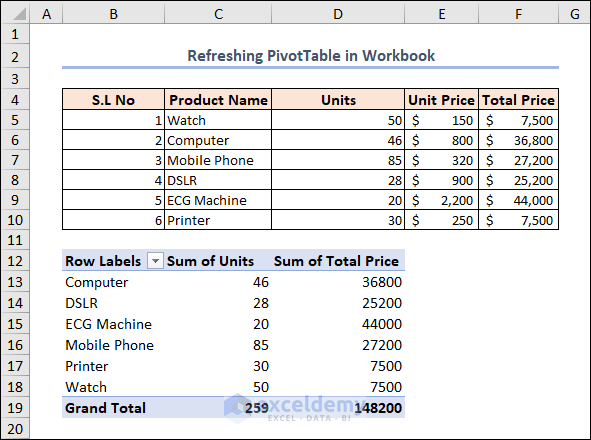
If we change the D7 cell value from 85 to 90, the total price in the F7 cell is updated below according to the respective changing value. But, in the PivotTable, no change occurs.

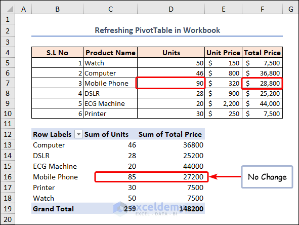
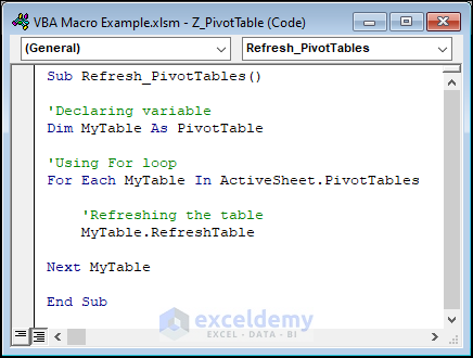
The following code will update the pivot table.

Sub Refresh_PivotTables()
'Declaring variable
Dim MyTable As PivotTable
'Using For loop
For Each MyTable In ActiveSheet.PivotTables
    'Refreshing the table
    MyTable.RefreshTable
Next MyTable
End Sub

If your workbook contains multiple pivot tables, you can use this code to update them all at once.

After running the above macro code, it will show the updated value in the PivotTable according to our corresponding dataset.

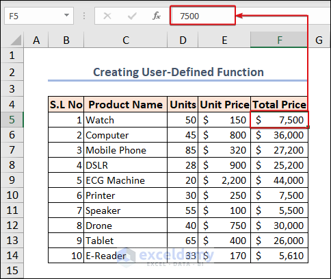
Example 25 – Creating a User-Defined Function

To calculate the total price, we can build a custom function that will be used like any other Excel function. Here’s the code.

Function Total_Price(x As Long, y As Long) As Long
'Using Product formula
Total_Price = x * y
End Function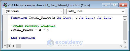

The following macro will directly calculate the output.

Sub Calculate_Total_Price()
Dim LRow As Long
Dim i As Long
'Get the last row of data in column B
LRow = Cells(Rows.Count, 2).End(xlUp).Row
'Loop through each row of data
For i = 5 To LRow 'Starting from row 5 because row 1 to 4 are header rows
    'Calculate the total price using the _
    Total_Price function and insert the value in column F
    Cells(i, 6).Value = Total_Price(Cells(i, 4).Value, Cells(i, 5).Value)
Next i
End Sub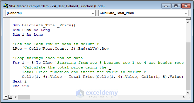

We can get the total prices in Column F in our sheet. Clicking on the cells in the F5:F14 range will show that no formula or function is showing in the cell. We added value directly through the VBA code.

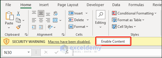
How to Enable Macro in Excel?

Clicking the Enable Content button on the yellow security notification bar that shows at the top of the sheet when you initially access a workbook with macros is the simplest and fastest way to enable macros for a single workbook.

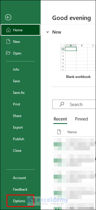
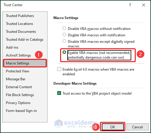
How to Change the Macro Settings from Trust Center?

• Click on File and select Options.

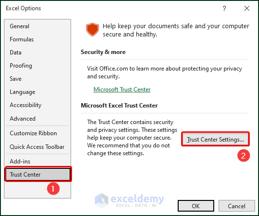
• From the Excel Options dialog box, select Trust Center and go to Trust Center Settings.

• Select Macro Settings and choose Enable VBA macros option.
• Click OK.

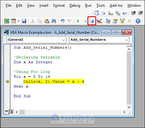
How to Test and Debug VBA Macro Code

You can easily test and debug a macro using the F8 key on the keyboard. You can then see the impact of each line on your worksheet as you go through the macro code line by line. Yellow highlighting indicates the line that is presently being run.

Press the Reset button on the toolbar to get out of debug mode.

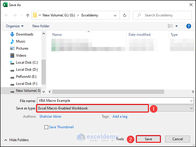
How to Save VBA Macro in Excel

• Press Ctrl + S keyboard shortcut command to save any file.
• In the Save As dialog box, choose Excel Macro-Enabled Workbook format in the Save as type field and click on the Save button.

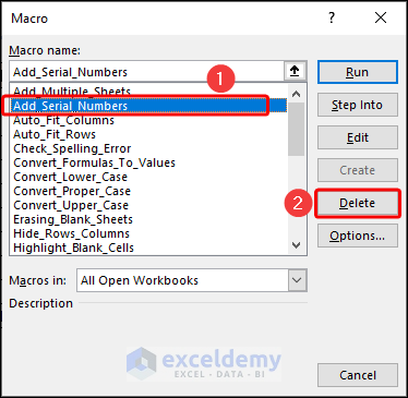
How to Delete Macro from Excel

• Go to Macros in the Developer tab.
• Select the macro you want to delete and click on the Delete button.

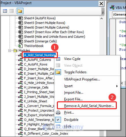
Alternatively:

• Open the VBA window.
• Right-click on the module name in Project Explorer.
• Select Remove.

Things to Remember

• Always save a backup copy of your Excel file before making any changes to it with the VBA code.
• When writing VBA code, use comments to explain what your code does. This will make it easier for you (and others) to understand the code in the future.
• Use meaningful variable names to make your code easier to read and understand.
• Be aware of the limitations of VBA macros. Some Excel features may not be accessible through VBA, and there may be performance issues with very large data sets.

Frequently Asked Questions

Can I record a macro in Excel?

You can use the macro recorder in Excel to record a series of actions and generate VBA code based on those actions. However, the resulting code may not be as efficient or customizable as handwritten code.

Can VBA macros be used in other Microsoft Office applications?

Yes, you can use VBA macros in other Microsoft Office applications, such as Word and PowerPoint. However, the specific VBA code required may differ depending on the application.

Are VBA macros secure?

VBA macros can pose security risks if they aren’t created or used properly. Macros can potentially contain malicious code, so it’s important to enable macro security settings in Excel and only run macros from trusted sources.

What are some common uses for VBA macros in Excel?

You can use VBA macros for a variety of tasks in Excel, such as automating data entry, formatting reports, creating custom functions, and manipulating data. Some common examples include automating financial models, generating charts and graphs, and performing data analysis.

Download the Practice Workbook

Related Articles

• How to Save VBA Code in Excel
• Using Macro Recorder in Excel
• How to Record a Macro in Excel
• How to Edit Macros in Excel
• How to Remove Macros from Excel
• How to Save Macros in Excel Permanently
• How to Use Excel VBA to Run Macro When Cell Value Changes
• Excel VBA to Pause and Resume Macro
• Excel Macro Enabled Workbook