This article demonstrates how to make a side-by-side Comparison Chart in Excel. A Comparison Chart is a handy tool in a variety of situations. In Excel, there is no such type of default chart named Comparison Chart. But you can make a Comparison Chart with the help of other chart types. Here, we will take you through 6 easy and convenient examples of creating a side-by-side Comparison Chart in Excel.
Side-by-Side Comparison Chart in Excel: 6 Examples
Suppose you have the following dataset. It includes the Price Comparison of three different Brands in five different States.

Now, we’ll make a side-by-side Comparison Chart using various methods from this dataset above.
1. Side by Side Comparison with Line Chart

Follow the steps below to create a side-by-side Comparison Chart of the prices of different brands in different states.
Steps:
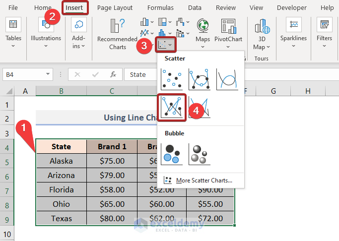
- At first, select cells in the B4:E9 range.
- Then, go to the Insert tab.
- After that, click on the Insert Scatter (X, Y) or Bubble Chart.
- Next, choose the Scatter with Straight Lines and Markers from the available charts.
- At this moment, you will get the following result.
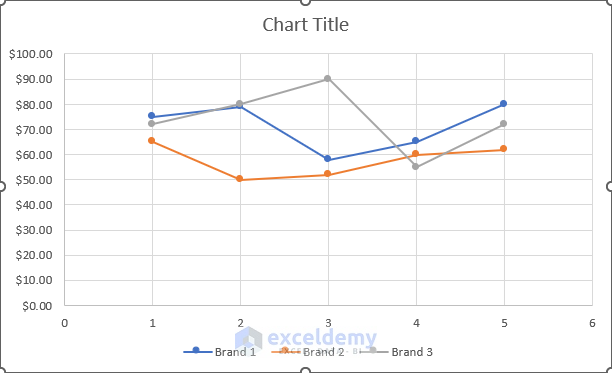
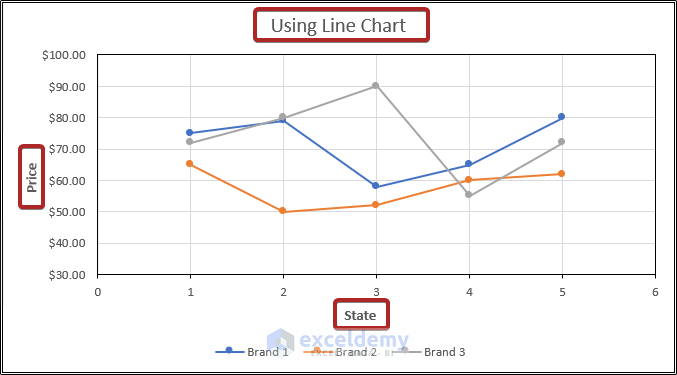
- Now, you can add Axis Titles, Chart Title. Also, you can edit them easily.
Read More: How to Create Weekly Comparison Chart in Excel
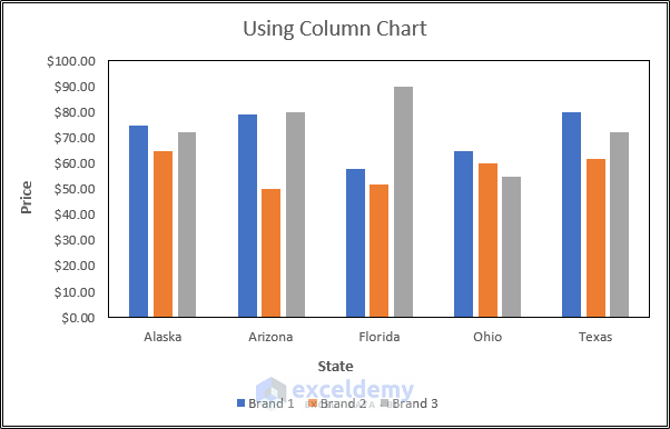
2. Side by Side Comparison with Column Chart

Similarly, you can present the side-by-side comparison with the Column Chart. Follow the steps below.
Steps:
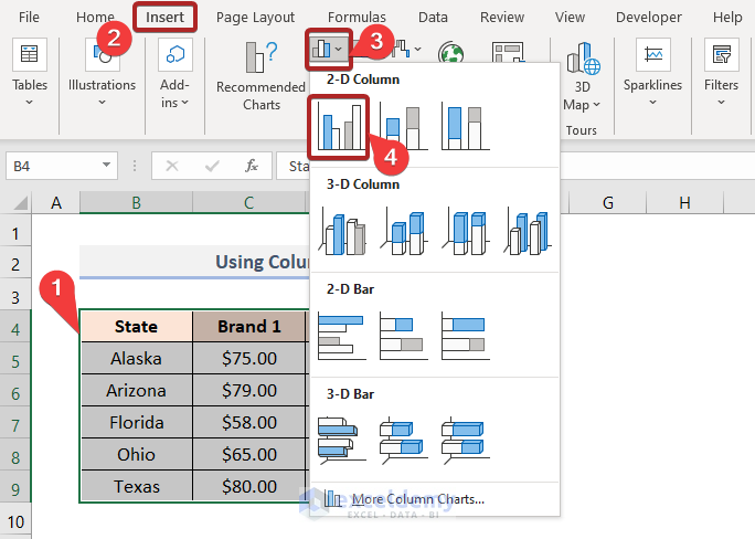
- Initially, select cells in the B4:E9 range.
- Then, move to the Insert tab.
- After that, click on the Insert Column or Bar Chart.
- Next, choose the 2-D Clustered Column from the available charts.
- At this point, the Column Chart is inserted as follows.
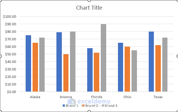
- Next, add Axis Titles and edit the Chart Title.
Read More: How to Create Quarterly Comparison Chart in Excel
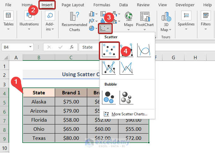
3. Side by Side Comparison with Scatter Chart

A Scatter Chart is also a very good way to represent a side-by-side Comparison Chart. In a Scatter Chart, you will not have texts on the horizontal axis. Rather, it will show the States on the horizontal axis as numerical values. Keeping this in mind, if you want to make a side-by-side Comparison Chart in Excel, you can follow the below steps.
Steps:
- At the very beginning, select the whole dataset. In this case, we select cells in the B4:E9 range.
- Second, go to the Insert tab.
- Then, select Insert Scatter (X, Y) or Bubble Chart.
- Next, click Scatter to insert a Scatter Chart.
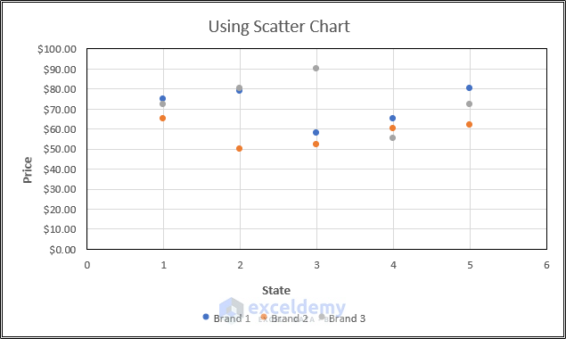
- Subsequently, edit the Chart Title and add Axis Titles.
- Finally, you will get the chart as shown below.
Read More: How to Create Month-to-Month Comparison Chart in Excel
4. Side by Side Comparison with Bar Chart

The Bar Chart is also like the Column Chart. However, their orientation is what makes them different. The sole distinction is that the Column Chart is displayed vertically (with values on the y-axis and categories on the x-axis), whilst the Bar Chart is presented horizontally (with values on the x-axis and categories on the y-axis).
To make a Bar Chart for side-by-side comparison in Excel, follow our steps below.
Steps:
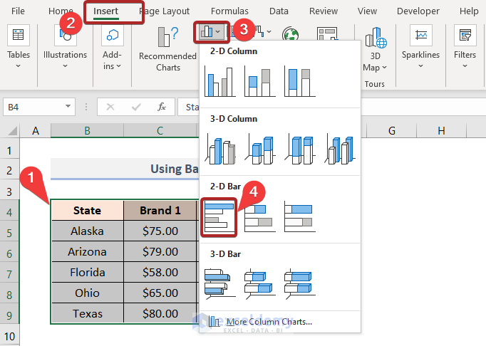
- Firstly, select cells in the B4:E9 range.
- Secondly, go to the Insert tab.
- Then, select Insert Column or Bar Chart.
- After that, choose 2-D Clustered Bar from the available options.
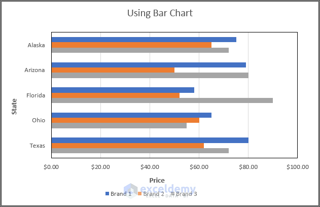
- Afterward, edit the Chart Title and add Axis Titles.
- Finally, you will get the chart as shown below.
Read More: Year Over Year Comparison Chart in Excel
5. Side by Side Comparison with Pivot Chart
Another alternative to create a side-by-side Comparison Chart in Excel is to insert a Pivot Chart. Follow the steps below to be able to do that.
Steps:
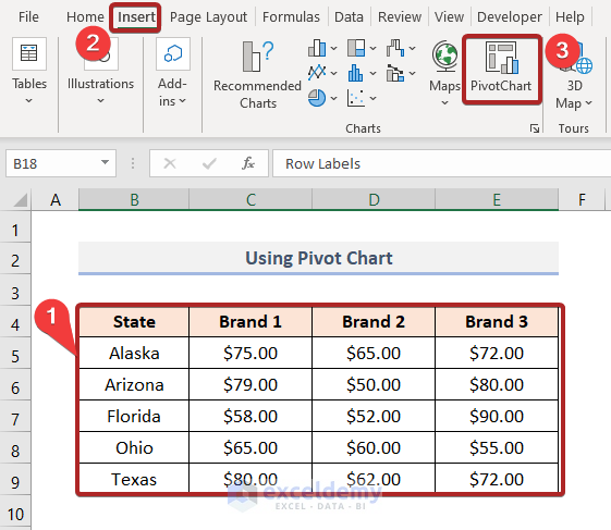
- First, select the dataset as we selected cells in the B4:E9 range here.
- Secondly, move to the Insert tab.
- Then, choose PivotChart from the Charts group.
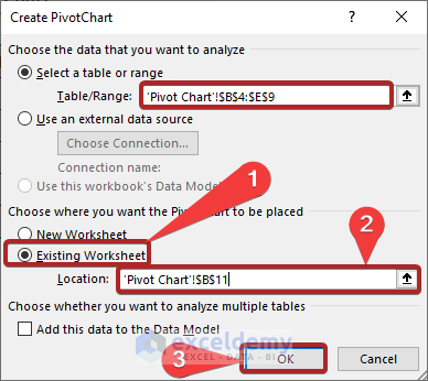
In this way, the Create PivotChart dialog box will appear.
- Then, choose Existing Worksheet to place our Pivot Chart.
- After that, select cell B11 as the placing Location.
- Afterward, click OK.
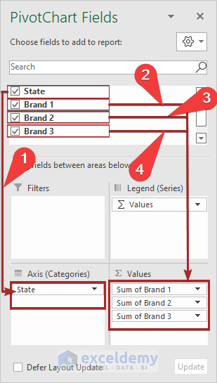
Now, the PivotChart Fields task pane opens on the right side of the display.
- Then, drag down State to the Axis (Categories) and Brand 1, Brand 2, and Brand 3 to the Values area.
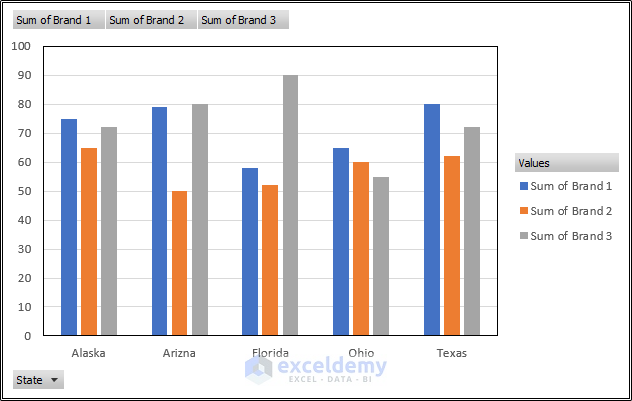
- At this moment, the Pivot Table looks like below.

- Besides, our chart also looks like the one below.

Read More: How to Use Comparison Bar Chart in Excel
6. Inserting Combo Chart

Now, we are going to create a side-by-side Comparison Chart using the Combo Chart feature of Excel. Follow our steps below.
Steps:
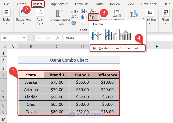
- Firstly, select the dataset and then go to the Insert tab.
- After that, select Insert Combo Chart.
- Later, click on Create Custom Combo Chart from the drop-down.
At this moment, the Insert Chart window opens.
- Already, we selected Combo before.
- Now, click OK.
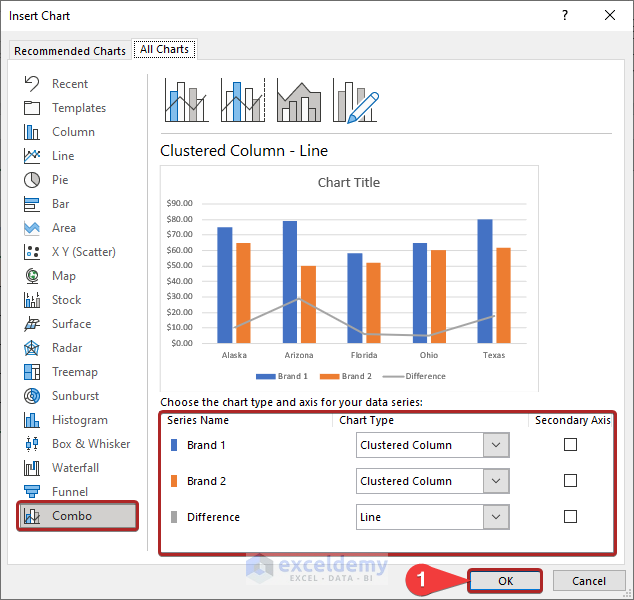
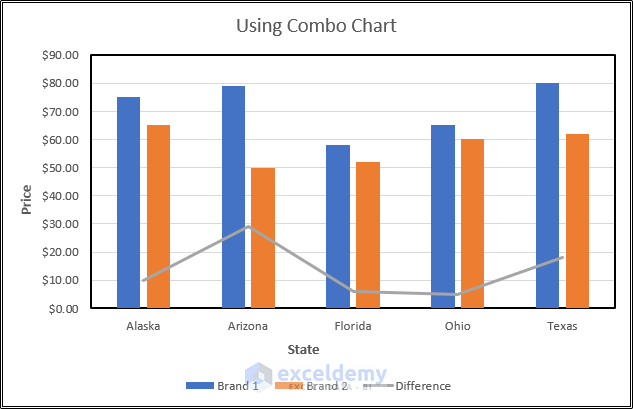
- Hence, the Combo Chart looks like the one below.
- It compares the price of two different brands using the Column Chart. Also, it displays the difference between the price of the two brands with a Line Chart.
Download Practice Workbook
You may download the following Excel workbook for better understanding and practice yourself.
Conclusion
Thank you for reading this article, we hope this was helpful. Please let us know in the comment section if you have any queries or suggestions. Please visit our website Exceldemy to explore more.
<< Go Back to Comparison Chart in Excel | Excel Charts | Learn Excel
Get FREE Advanced Excel Exercises with Solutions!

Pal, i cannot solve a problem myself. Can you sort it out for me? I works in a depot. Our employees sell the products. I have to submit my boss a chart of their sales.like, in first column have the employee name, next the sales of april,in next two colums there are sales for may & june. I want to make a chart where x axis gets the month name and y axis has the total sales. But excel inserts chart for each employee and their monthly sales in different colums. Got it? It would be very nice if you solve it for me.
Hello ROMA,
Sorry for being late. And we love to solve our user’s problems.
First of all, download the Practice Workbook for your own convenience.
• At the very beginning, we’ve made a relevant dataset for your problem.
• Then, make a new row in Row 9 with the heading Total Monthly Sales. Also, a new column Total Sales in Column F.
• Later, select cell C9 and enter the formula below.
=SUM(C5:C8)• Next, press ENTER.
• Alternatively, press ALT+= on the keyboard as a shortcut to do the same task.
• Now, get the cursor to the bottom-right corner of cell C9; instantly, it will look like a plus (+) sign. Actually, it’s the Fill Handle tool.
• Thus, drag it to the right corner of cell E9.
Therefore, we get the desired results in other cells too.
• Similarly, go to cell F5 and paste the following formula.
=SUM(C5:E5)• As usual, press ENTER.
Currently, we’ll insert the chart.
• Firstly, go to the Insert tab.
• Secondly, click on Insert Column or Bar Chart dropdown on the Charts group.
• Thirdly, select 2-D Clustered Column from the available options.
As a result, we can see a blank chart on the worksheet.
• Then, right-click anywhere on the chart area.
• It opens a context menu. Hence, choose Select Data from the options.
Immediately, the Select Data Source dialog box opens.
• Here, click on the Add button under the Legend Entries (Series) section.
Instantly, the Edit Series input box appears.
• Then, give the Series name as Monthly Sales.
• In the box of Series values, give the reference of the C9:E9 range.
• After that, click OK.
• Thenceforth, click on the Edit button under the Horizontal (Category) Axis Labels.
• Following this, give the reference of the C4:E4 range in the Axis label range box.
• After that, click OK.
It returns us to the Select Data Source dialog box again.
• Next, press the OK button.
Simply, a column chart will be visible on the worksheet. It includes the month-wise sales amount.
• Hereafter, add Axis Titles and Legend to the chart using the Add Chart Element option.
Now, we’ll create the second chart as per your question.
• Similarly, insert another blank chart and open the Select Data Source dialog box.
• Then, click on Add.
• Then, in the Edit Series dialog box, do the following as in the image below.
• Also, change the Horizontal Axis Labels like before.
• After that, click OK.
Here is the desired chart of employee-wise total sales.
• Bring some edits to the chart to make it more appealing.
I have another question also. Forget to mention earlier. Is it possible to get the same chart with employee in x axis and total sales in y axis.???
It is so urgent. Can you mail the solution please?