How to Create Weekly Comparison Chart in Excel

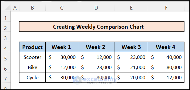
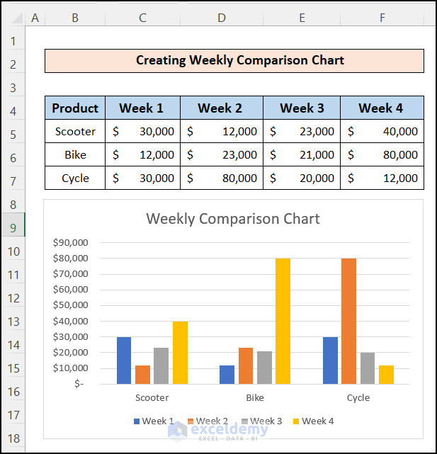
Step 1 – Create a Dataset

• Create a dataset to create a weekly comparison chart in Excel. We have created a dataset with sales data for 3 products over 4 weeks.

Step 2 – Insert a Column Chart

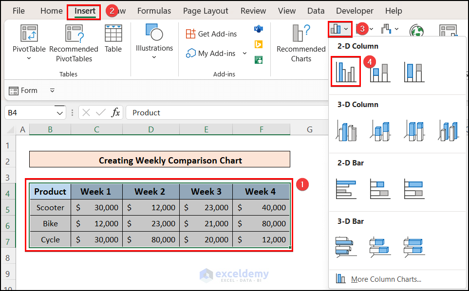
• Select the dataset.
• Go to the Insert tab on the top ribbon.
• Click on the Bar Chart icon and select a 2D Column Chart from the list.

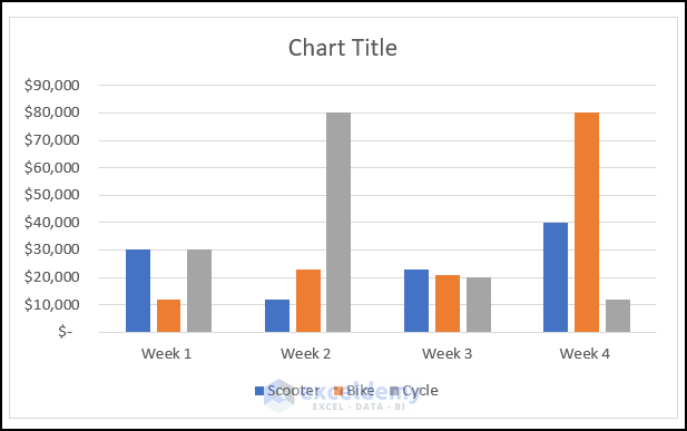
• You will see a Bar chart created showing the weekly comparison for each product.

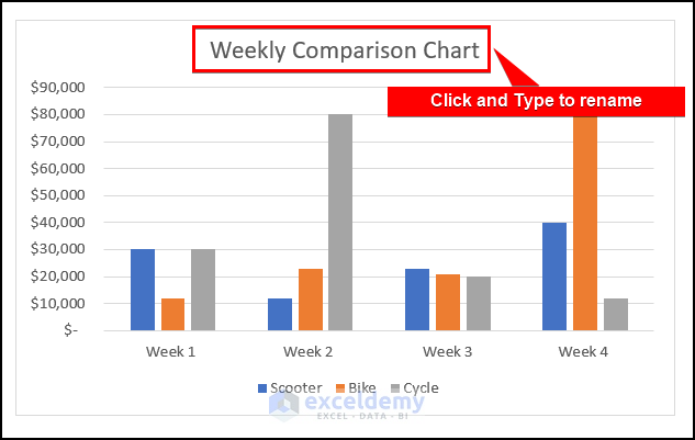
Step 3 – Give a Title to the Chart

• Double-click on the chart title and rename it.

Read More: How to Create Quarterly Comparison Chart in Excel

Final Step – Switch the Rows and Columns of the Chart

• Click on the Chart.
• Go to the Chart Design
• Click on Switch Row / Column

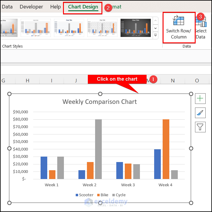
• The chart is transformed and shows a weekly comparison of sales of each product individually.

Read More: How to Use Comparison Bar Chart in Excel

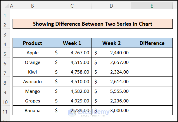
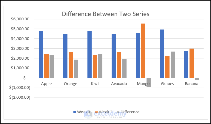
Excel Chart to Show Differences Between Two Series

Steps:

• Create the dataset and a new column to calculate the difference between the columns.

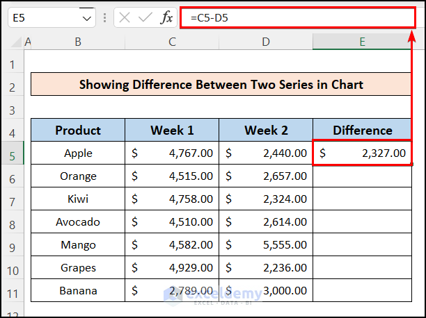
• Insert the following formula into cell E5 to calculate the difference between cells C5 and D5

• AutoFill the formula down.

• Select the full dataset including the difference column and create a bar chart.
• You can easily visualize the comparison of the selling price, cost price, and difference of prices of each product individually.

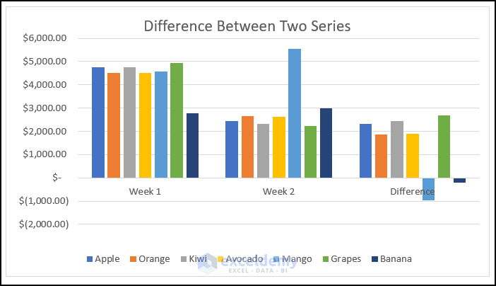
• You can click on the Switch Row/Column to show the selling price, cost price, and differences of all products individually.

Download the Practice Workbook

Related Articles

• How to Create Month to Month Comparison Chart in Excel
• Year Over Year Comparison Chart in Excel

<< Go Back to Comparison Chart in Excel | Excel Charts | Learn Excel