How to Create a Budget vs an Actual Chart in Excel – 2 Methods

What Is Budget vs Actual Chart?

A budget vs actual chart is used to determine the difference or variance between the forecast and actual value.

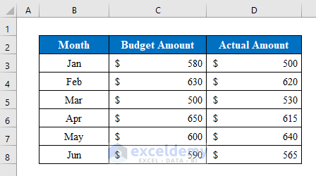
The dataset showcases the Budget Amount and the Actual Amount monthwise. To create a budget vs actual chart:

Method 1 – Use Bars to Create a Budget vs Actual Chart

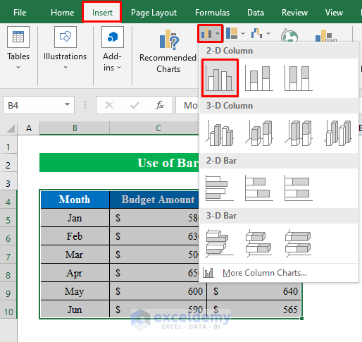
Step 1:

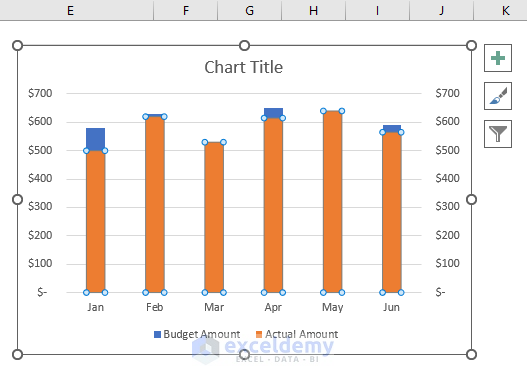
• Select the data and choose “2-D Column” in “Insert”.

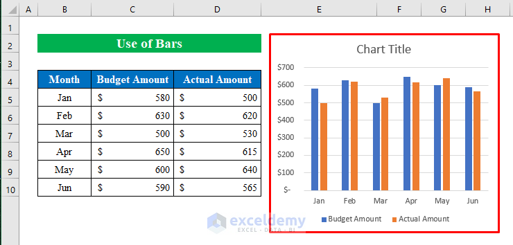
• A chart is created in your worksheet.

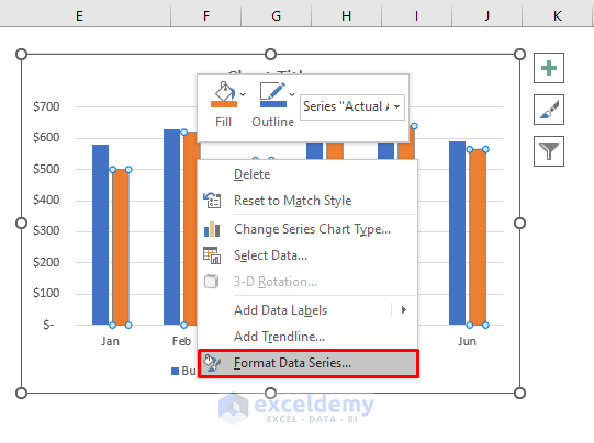
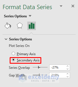
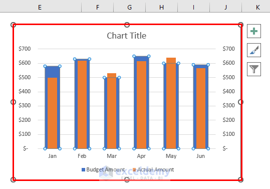
• Right-click and choose “Actual Value Bar”.
• Select“Format Data Series”.

• Click “Secondary Axis”.

• This is the output.

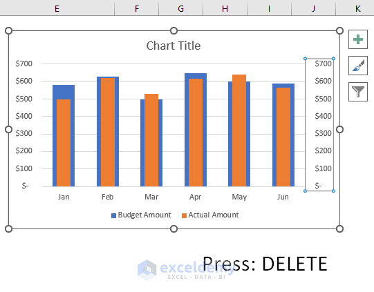
Step 2:

• To edit the “Budget Bars” , select it and choose “Format Data Series”.

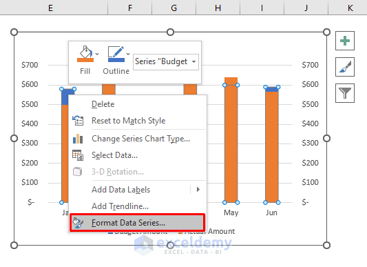
• Change the “Gap Width” to “100%”.

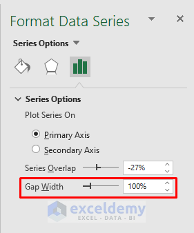
• This is the output.

Step 3:

• To remove the horizontal axis value, select values and press DELETE.

• To change the format, select the chart and click “Format Data Series”.

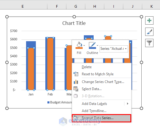
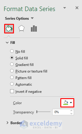
• Choose “Fill” feature and select a color.

• Change the “Chart Title”.
• This is a budget vs actual chart in Excel.

Read More: How to Make a Price Comparison Chart in Excel

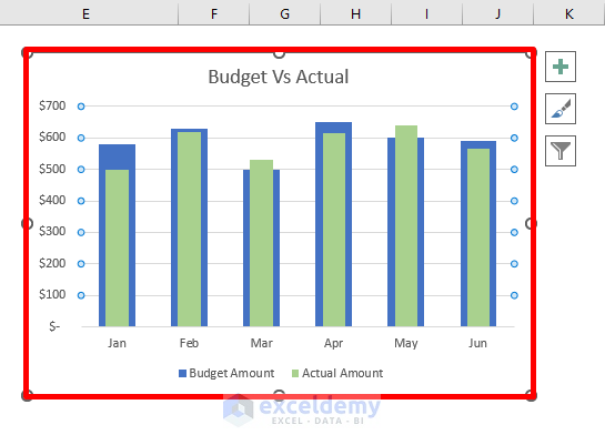
Method 2 – Use Marker Lines to Create a Budget vs Actual Chart

Step 1:

• Select the data and choose “2-D Column” in “Insert”.

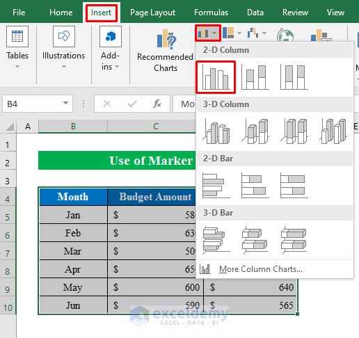
• A chart will be  automatically created.
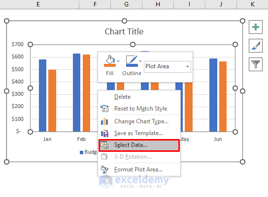
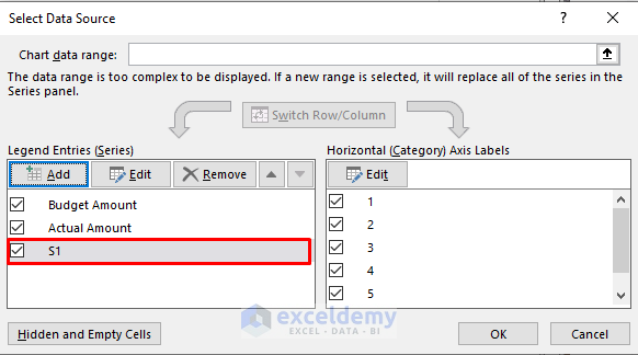
• Select the chart and click “Select Data” to add data.

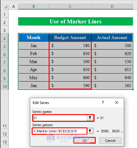
• Click “Add”.

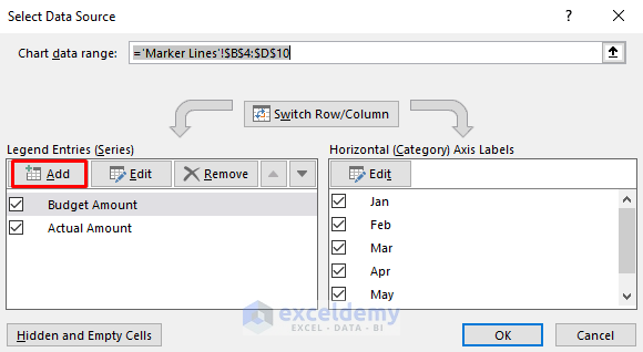
• In “Edit Series”, provide a “Series Name”.
• In “Series values”, choose “Budget Amount”.

• A new series was added to the chart.

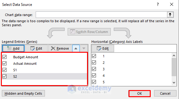
• Add another data series with the “Actual Amount” value.
• Click OK.

Step 2:

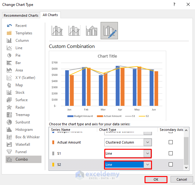
• Edit the series by selecting a bar and clicking “Change Series Chart Type”.

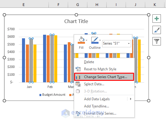
• Select “Line” for “S1” and “S2”.
• Click OK.

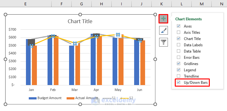
• In “Chart Elements”, check “Up/down Bars”.

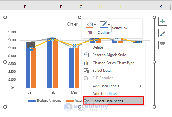
• Add and edit the marker by selecting “Format Data Series”.

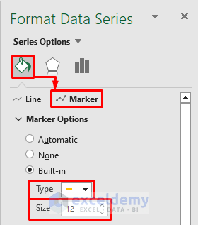
• Choose “Marker” in “Fill”.
• Choose a format in “Type” and change the size in “Size’

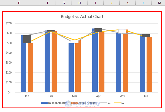
• The budget vs actual chart is displayed.

Read More: How to Compare 3 Sets of Data in Excel Chart

Download Practice Workbook

Download the practice workbook to exercise.

Related Articles

• How to Make Sales Comparison Chart in Excel
• How to Make a Salary Comparison Chart in Excel
• How to Make a Comparison Chart in Excel
• How to Compare Two Sets of Data in Excel Chart

<< Go Back to Comparison Chart in Excel | Excel Charts | Learn Excel