How to Use Sheet Name Code in Excel (4 Applications)

In this article, we will learn how to use and get sheet name code in Excel. In Microsoft Excel, we can use the sheet name directly in a formula as a reference. We will go over different examples with the different datasets to illustrate the process of using sheet name code Excel.

How to Use Sheet Name Code in Excel: 4 Applications

In this tutorial, we will cover 4 applications of Excel sheet name code. We will use formulas, and VBA code to interact with sheet name code. Let’s dive into the process.

1. Excel Function to Insert Current Sheet Name Code

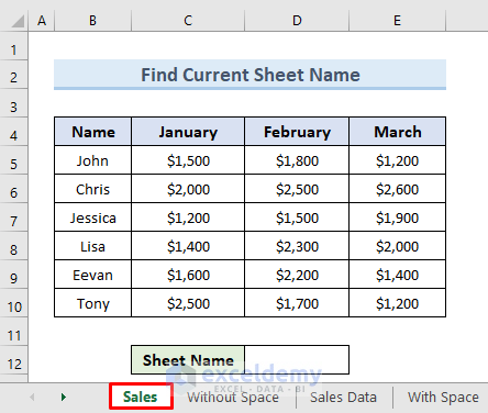
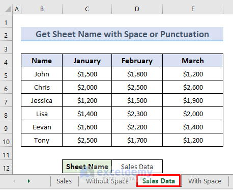
First and foremost, we have the following dataset of six salespeople. It tells us the number of sales for January, February, and March. In this example, we will find out the sheet name of the current sheet in cell D12.

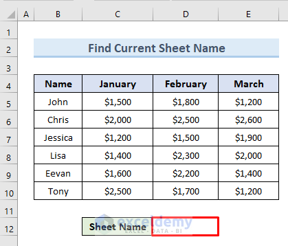
In the beginning, select cell D12.
Insert the formula in that cell.

=MID(CELL("filename",A1),FIND("]",CELL("filename",A1))+1,255)

Press Enter.
We get the name of the current sheet in cell D12.

🔎 How Does the Formula Work?

CELL(“filename”,A1))+1,255): This part extracts the full file name and path.
FIND(“]”,CELL(“filename”,A1))+1,255): As the text argument, CELL passes this result to the MID function. Because the sheet name begins right after the left bracket, the FIND function is used to determine the starting location.
MID(CELL(“filename”,A1),FIND(“]”,CELL(“filename”,A1))+1,255): Returns the name of the current worksheet. The maximum number of characters to extract is 255. You can’t name a worksheet longer than 31 characters in Excel. But the file format allows for worksheet names of up to 255 characters, therefore the complete name is received.

2. Use Sheet Name Code as Reference in Excel Formula

2.1 Without Spaces or Punctuation Characters

For this example, we will have to look at our previous dataset. The sheet name of our previous dataset is Sales. If you notice that there is no punctuation or spaces in the sheet name. In this example, we will use sheet names without punctuation or spaces as a reference in another worksheet. We will use the INDIRECT function to do this task. The following figure is just an overview of our previous dataset.

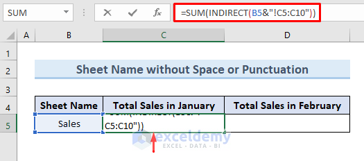
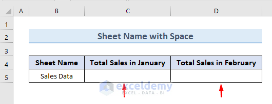
Now, look at the below image. Our purpose for this example is to calculate the total sales amount of January of our previous dataset. We will input the total value in cell C5.

Select cell C5 and insert the following formula.

=SUM(INDIRECT(B5&"!C5:C10"))

Then, hit Enter.

Finally, we get the total sales amount for January in cell C5.

Again we can get the total sales for February by inserting the following formula in cell D5.

=SUM(INDIRECT(B5&"!D5:D10"))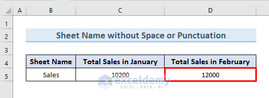

🔎 How Does the Formula Work?

INDIRECT(B5&”!C5:C10″): This part considers the sheet name in cell B5. Then, take the values of the range C5:C10 from that sheet.
SUM(INDIRECT(B5&”!C5:C10″)): Returns the value of range C5:C10.

2.2 With Spaces or Punctuation Characters

In our previous example, we didn’t have any spaces or punctuations in our sheet name. For this example from the following dataset, we can see that we have a space between two words in our sheet name. The name of the sheet is Sales Data. Let’s see which problems we face for this space to use this as a reference. Also, we will look at how we can solve this problem.

Here, we will calculate the total amount of sales for the months of January and February.

First, select cell C5 and insert the formula that we used in our previous example.

=SUM(INDIRECT(B5&"!C5:C10"))

Press Enter.
We get the #REF! error.

Now there might be a question in your mind. We are doing the same process as our previous example. Why is it showing an error? It’s because of the space in the name of the worksheet. Our formula does not read after space. As a result, it does not find any match for the worksheet and shows an error.

Now to solve this problem insert the following formula. The new formula is slightly different from the previous one.

=SUM(INDIRECT("'"&B5&"'!C5:C10"))

Press Enter.
We can see the total sales amount for the month of January in cell C7.

Similarly, by inserting the following formula we get the total sales amount for the month of February.

=SUM(INDIRECT("'"&B5&"'!D5:D10"))

3. VBA to Get Sheet Name Code in Excel

Using VBA(Visual Basics for Applications) code, we can get sheet name code easily. In this section, we will see the use of VBA code to extract sheet names.

3.1 Find Active Sheet Name

We can find the name of the active worksheet with VBA. For this example, we have the following dataset. We will extract the name of this sheet in cell D12.

Now to step further you will need the Developer tab in the menu bar to make macro-enabled content. If you do not have the Developer tab in your Excel menu bar, follow the steps below to get the Developer tab. If you already have the Developer tab in your Excel just skip this part and continue from next. Let’s see how we can make the Developer tab visible.

Go to the File option in the top-left corner of our Excel.

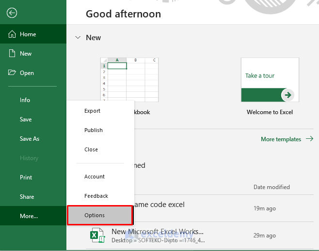
Next, select the Options.

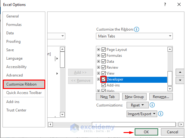
Then, a new window will come. Select the option Customize Ribbon from the available options.
Select the Developer option and click OK.

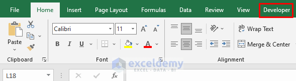
Finally, we can see the Developer tab in our Excel.

Now we will use the Developer tab to create macro-enabled content. Let’s see how we can do this in the following steps.

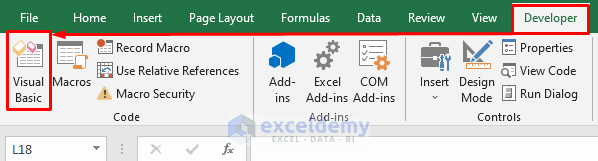
Go to the Developer tab.
Then, select the Visual Basic option.

Here, a new window will open. From the window select the Insert tab.
From the drop-down, select the Module option.

Select the option Module-1. A blank window will open.

Then insert the following code in the blank window.

Sub SheetName()
Range("D12") = ActiveSheet.Name
End Sub

We will click on the Run option from the main tab. Also, we can press F5 to run the code.

Finally, we can see the name of the active sheet in cell D12.

3.2 Input All Sheet Names in Cells Using VBA

In this example, we will list all the worksheets of a workbook in a single worksheet using VBA code. In the following figure, we can see a worksheet named Sheet_List. We will list down all the worksheet names in column B of this sheet.

Open a new module for the worksheet.
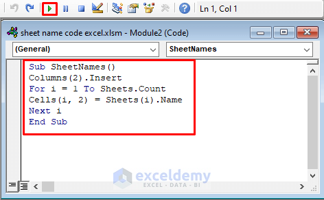
Next, insert the following code in the code window.

Sub SheetNames()
Columns(2).Insert
For i = 1 To Sheets.Count
Cells(i, 2) = Sheets(i).Name
Next i
End Sub

Then click on the Run icon. We can also run the code by pressing the F5 key.

Finally, we can see the list of all sheets of this workbook in column B.

3.3 Use Code Number to Extract Sheet Name in Excel

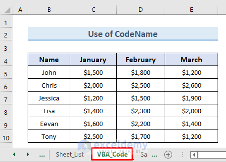
We can get the name of a sheet by using the CodeName of that sheet in the VBA code window. We will extract the sheet name of the following dataset by using the CodeName.

Open a new module for the worksheet.
Next, input the following code in the code window.

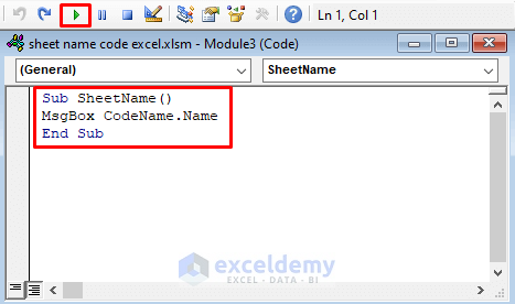
Sub SheetName()
MsgBox CodeName.Name
End Sub

Then click on the Run icon. We can also run the code by pressing the F5 key.

At last, we can see a new message box showing the name of the active sheet.

4. Insert Excel Sheet Name Code in Header and Footer

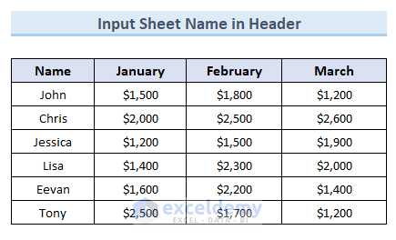
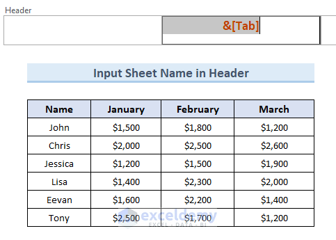
In this method, we will add sheet names in the header and footer sections of a worksheet. We will use the following dataset to illustrate this method.

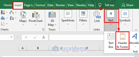
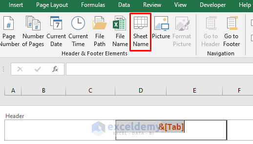
Go to the Insert tab.
Next, select the Text option. From the drop-down select the Header & Footer option.

Then, we will see a header section with a default text &[Tab].

After that, select the option Sheet Name from the Header & Footer Elements section.

Finally, we can see the name of the worksheet Sales Data Header in the header section.

Now like in this example, we will add the sheet name code in the footer section of the following dataset.

Go to the Header & Footer section.
Next, select the Footer option and select Sheet Name option.

Finally, we can see the sheet name Sales Data Footer in the footer section of the dataset.

Download Practice Workbook

You can download the practice workbook from here.

Use of Sheet Name Code.xlsm

Conclusion

In the end, we have gone through the different methods to use sheet name code Excel in this article. To practice yourself download the practice workbook added with this article. If you feel any confusion just leave a comment in the below box. We will try to answer as soon as possible. Stay tuned with us for more interesting solutions to Microsoft Excel problems.