How to List Sheet Name in Excel (5 Methods + VBA)

In this article, we’ll discuss various ways to derive a list of sheet names in Excel. Unfortunately, there is no dedicated function to fetch a list of sheet names in Excel, but we can use a combination of several functions, the 2-step process of using Name Manager & formula, or VBA code to retrieve a list of sheet names into a single column.

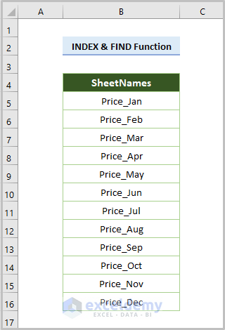
In the following figure, we have 12 sheets which are mainly prices in months during a year. The names of the sheets are Price_Jan, Price_Feb, and so on.

Dataset

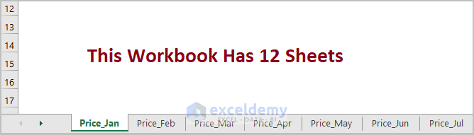
Let’s fetch a list of the sheet names.

Method 1 – Using the Combination of INDEX & FIND Functions

We can use a formula containing the INDEX, LEFT, MID, and FIND functions.

Steps:

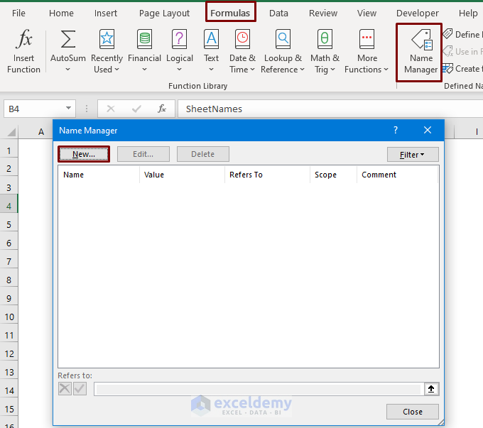
Click on the Formulas tab > Select the Name Manager option from the Defined Names ribbon.
In the Name Manager box that opens, click the New button.

Opening Name Manager

Insert the Name (here, Worksheets).
Insert the below formula in the Refers to section:

=GET.WORKBOOK(1)&T(NOW())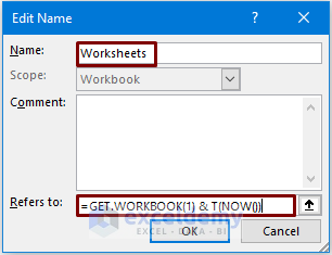

Creating a New Name

Note:
GET.WORKBOOK is a macro-enabled function that stores the sheet names in the workbook.

Enter the following formula in cell B5:

=INDEX(MID(Worksheets,FIND("]",Worksheets)+1,255),ROWS($B$5:B5))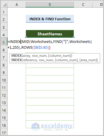

Sheet Name List Using INDEX & FIND Functions

Press Enter and use the Fill Handle tool to fill the cells below.

The list of sheet names is returned.

Sheet Name List Using INDEX & FIND Functions

Method 2 – Using the INDEX and REPLACE Functions (Automated List)

This time, after clicking the New option from the Name Manager dialog box, insert the Name as SheetNames, and the below formula in the Refers to section:

=REPLACE(GET.WORKBOOK(1),1,FIND("]",GET.WORKBOOK(1)),"")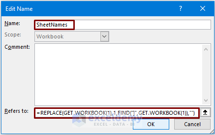

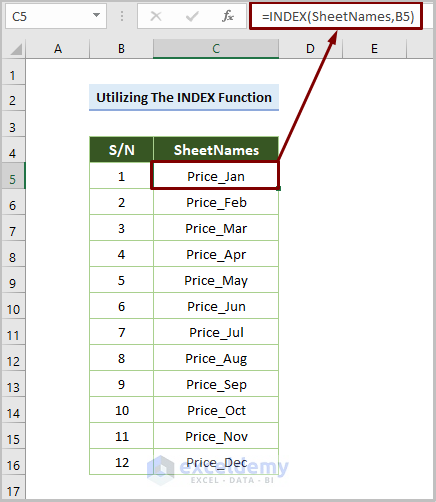
Sheet Name List Utilizing The INDEX Function

Insert the following formula in cell C5:

=INDEX(SheetNames,B5)

B5 is the starting cell of the serial number (S/N).

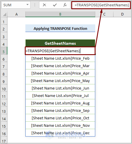
Sheet Name List Utilizing The INDEX Function

Method 3 – Using the TRANSPOSE Function

The TRANSPOSE function returns a horizontal cell range as a vertical cell range, or vice versa.

Steps:

Ensure the Name is GetSheetNames.
Enter the below formula:

=GET.WORKBOOK(1)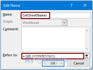

Applying TRANSPOSE Function to Find The Sheet Name List

Insert the following formula:

=TRANSPOSE(GetSheetNames)

The following output is returned:

Applying TRANSPOSE Function to Find The Sheet Name List

Method 4 – Using the LOOKUP Function

Before using the LOOKUP function, create a new name where the Name is Sheets and the formula in the Refers to section is:

=GET.WORKBOOK(1)&T(NOW())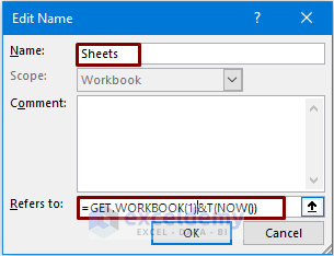

Using the LOOKUP Function to Get the Sheet Name List

Note:
The same macro-enabled formula is used as in the first method (Name: Worksheets).

Insert the formula:

=LOOKUP("xxxxx",CHOOSE({1,2},"",INDEX(MID(Sheets,FIND("]",Sheets)+1,255),ROWS(B$1:B1))))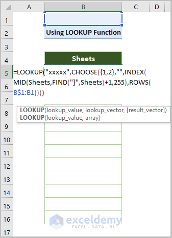

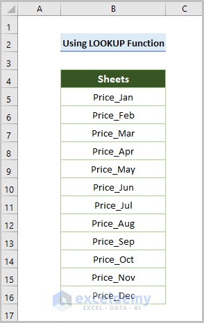
Excel Sheet Name List Using the LOOKUP Function

Press Enter and use the Fill Handle to return the following output:

Using the LOOKUP Function to Get the Sheet Name List

Method 5 – Dynamic List of Sheet Names Using SUBSTITUTE Function

We can create a dynamic list of sheet names using the SUBSTITUTE function.

Steps:

Set the name as Dynamic_List_of_SheetNames and enter the below formula:

=SUBSTITUTE(GET.WORKBOOK(1),"["&GET.WORKBOOK(16)&"]","")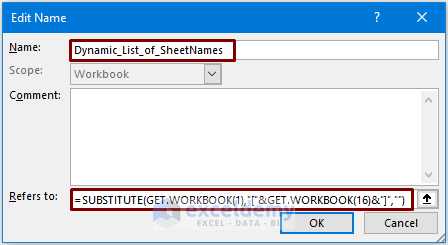

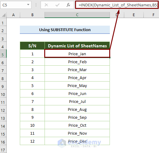
Creating a Dynamic List of Sheet Name Using SUBSTITUTE Function

Insert the following formula in cell C5:

=INDEX(Dynamic_List_of_SheetNames,B5)

B5 is the starting cell of the serial number (S/N).

Creating a Dynamic List of Sheet Name Using SUBSTITUTE Function

Method 6 – Using VBA Code

Last but definitely not least, we can apply VBA code to get the list of sheet names.

Steps:

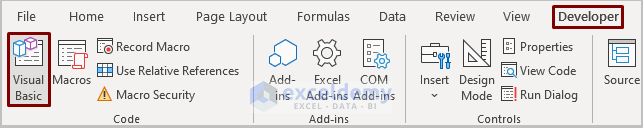
Open a module by clicking Developer > Visual Basic.

How to Insert VBA Code

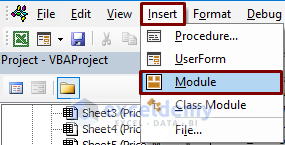
Go to Insert > Module.

How to Insert VBA Code

Copy and paste the following code into the module:

Sub GetListOfAllSheets()
   Dim w As Worksheet
   Dim i As Integer
   i = 5
   Sheets("Price_Jun").Range("B:B").Clear
   For Each w In Worksheets
       Sheets("Price_Jun").Cells(i, 2) = w.Name
       i = i + 1
   Next w
End Sub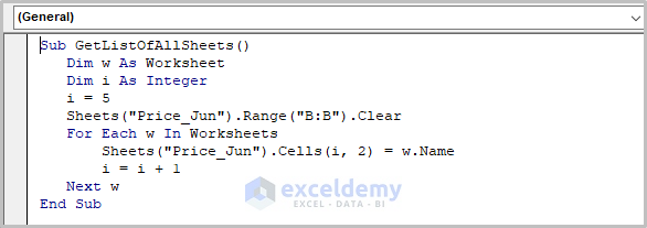

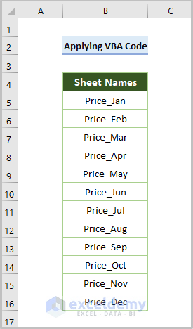
Sheet Name List Using VBA Code

Run the code.

The output will be as follows:

Sheet Name List Using VBA Code

Notes:
Take care of the following when using the VBA code:

Worksheet name: Here, the worksheet name is Price_Jun.
Cells(i, 2) means the cell location of row i (here, i=5) and column 2.

Things to Remember

I. As GET.WORKBOOK is a macro-enabled function, save the Excel file in .xlsm format (designated extension format for macro-enabled Excel file).

II. A #BLOCKED error may be returned instead of the output if the workbook is unable to update.

Download Practice Workbook

Sheet Name List.xlsm