When you work with an important dataset in your Excel including formulas, you need to protect those cells from being edited. Any alteration of your dataset can change the whole calculation. Excel gives you a useful platform where you can protect your dataset from being edited. This article will show you how to protect Excel cells from being edited with some useful examples. I hope you will enjoy the whole article and gain some valuable knowledge.
How to Protect Excel Cells from Being Edited: 6 Easy Methods
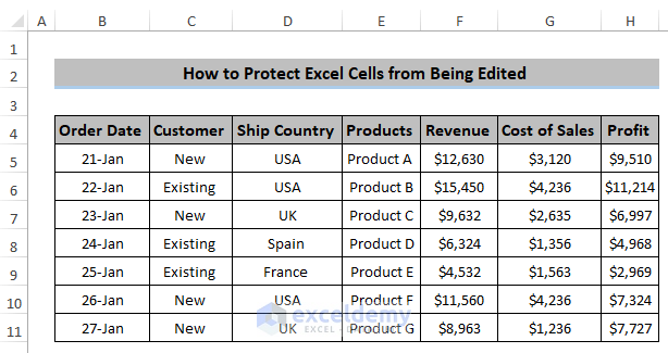
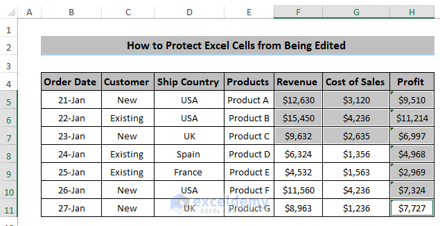
To protect Excel cells from being edited, we will show six different examples through which you have a clear idea about Excel cell protection. To do this, we take a dataset that includes Product revenue, cost of sales, and profit.
1. Protect All Cells from Being Edited
Firstly, you can protect all Excel cells from being edited. In this method, you need to lock the cells and apply the password to protect the sheet. By default, your cells are locked. But if it is not the case then lock it first and then apply for password protection. To do this follow the following steps carefully
Steps
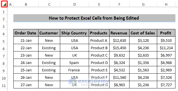
- First, you need to select all the cells by clicking the triangle where row and column headers coincide.
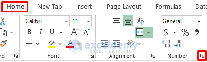
- Next, go to the Home tab in the ribbon and select Format Cells popup launcher or you can press Ctrl+1.
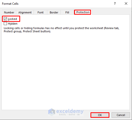
- A Format Cell dialog box will pop up. From there, select Protection.
- Next, check on the Locked option.
- Click on OK.
- Mind it, only locking in the Format Cells can’t make your Excel cells lock entirely. You need to protect the sheet with a password.
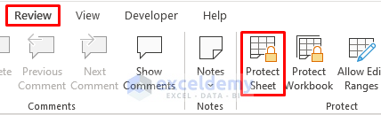
- Next, go to the Review tab and select Protect Sheet from the Protect group.
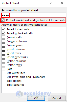
- A Protect Sheet dialog box will appear.
- After that, set any password in the password box.
- Check on the Protect worksheet and contents of locked cells.
- A Confirm Password dialog box will appear.
- Next, rewrite your given password.
- Finally, click on OK.

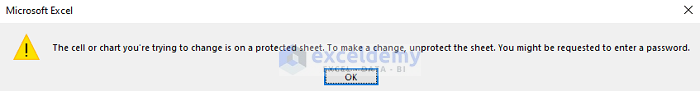
- After that, if you try to alter any cell in your worksheet, you’ll get the following message. See the screenshot.
Read More: How to Lock Multiple Cells in Excel
2. Protect Specific Cells from Being Edited
There are some cases where you need to protect specific cells. Those cells are really valuable that you don’t want anyone to alter this except you. In that case, you need to use this method.
Steps
- First, you need to unlock all the cells.
- Now, select all the cells by clicking the triangle where row and column headers coincide.
- Next, open the Format Cells by Pressing Ctrl+1.
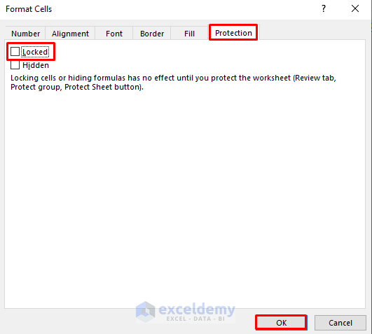
- After that, select the Protection option.
- Then, uncheck the Locked option.
- Finally, click on OK.
- Select some specific cells in your dataset. Select one cell first then press ‘Ctrl’ and select cells one after another. For adjacent cells, you can use ‘Shift’.
- Next, go to the Home tab in the ribbon.
- After that, select Format Cells popup launcher or you can press Ctrl+1.
- A Format Cell dialog box will pop up. From there, select Protection.
- Next, check on the Locked option.
- Click on OK.
- Go to the Review tab in the ribbon.
- Next, select Protect Sheet from the Protect group.
- A Protect Sheet dialog box will appear.
- After that, set any password in the password box.
- Then, check on the Protect worksheet and contents of locked cells.
- A Confirm Password dialog box will appear.
- Rewrite your given password.
- Click on OK.
- Now, try to alter the specified cells. Then you will find the following result. See the Screenshot.
Read More: How to Lock Certain Cells in Excel
3. Protect Specific Rows
Sometimes you need to protect specific rows from others. In some cases, you need to have some essential data in some specific data. If anyone alters this, your whole hard work will go in vain. In that case, you need to protect those specific rows from being edited. To apply this method, follow the following steps carefully.
Steps
- First, you have to unlock all the cells.
- Select all the cells by clicking the triangle where row and column headers coincide.
- Next, open the Format Cells by Pressing Ctrl+1.
- Select the Protection option.
- Uncheck the Locked option to unlock cells.
- Click on OK.
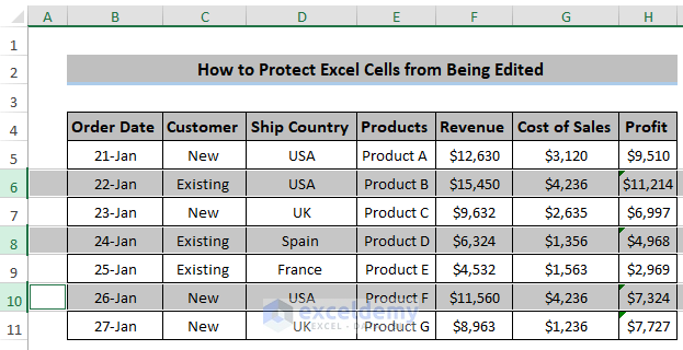
- Select some specific rows in your dataset. First, select any row and then press ‘Ctrl’ and select rows one after another.
- Next, go to the Home tab in the ribbon.
- Select Format Cells popup launcher or you can press Ctrl+1.
- A Format Cell dialog box will pop up. From there, select Protection.
- Next Check on the Locked option.
- Click on OK.
- Go to the Review tab in the ribbon.
- Select Protect Sheet from the Protect group.
- A Protect Sheet dialog box will appear.
- Set any password in the password box.
- Check on the Protect worksheet and contents of locked cells.
- A Confirm Password dialog box will appear.
- Rewrite your given password.
- Click on OK.
- Now, try to alter the specified rows. Then you will find the following result. See the Screenshot.
Read More: How to Protect Excel Cells with Password
4. Protect Excel Cells with Formulas
Sometimes you need to protect your excel cells which contain formulas. As an Excel regular user, it is known to all that if anyone alters your formula, it will change the whole worksheet. In our example, we need to protect our profit formula. To do this you need to follow the following steps carefully.
Steps
- First, you have to unlock all the cells.
- Select all the cells by clicking the triangle where row and column headers coincide.
- Next, open the Format Cells by Pressing Ctrl+1.
- Select the Protection option.
- Uncheck the Locked option to unlock cells.
- Click on OK.
- Next, you need to select the cells with formulas.
- Go to the Home tab in the ribbon.
- Select Find & Select from the Editing group.
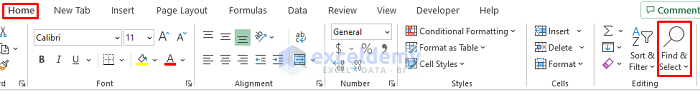
- Select Go To Special from Find & Select. See the screenshot.

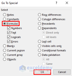
- A Go to Special dialog box will appear.
- Select Formulas.
- Click on OK.
- It will automatically select all the cells with applied formulas.

- Next, go to the Home tab in the ribbon.
- Select Format Cells popup launcher or you can Press Ctrl+1 as a keyboard shortcut.
- A Format Cell dialog box will pop up. From there, select Protection.
- Next Check on the Locked option.
- Click on OK.
- Go to the Review tab in the ribbon.
- Select Protect Sheet from the Protect group.
- A Protect Sheet dialog box will appear.
- Set any password in the password box.
- Check on the Protect worksheet and contents of locked cells.
- A Confirm Password dialog box will appear.
- Rewrite your given password.
- Click on OK.
- Now, try to alter the specified cells with formulas. Then you will find the following result. See the Screenshot.
Read More: How to Lock a Cell in Excel Formula
5. Using Allow Edit Ranges Command to Protect Cells
In this method, you can select the modifiable cells and other cells will be locked from editing. This method is useful for certain cases where you need to protect some specific cells. To use this method, follow the following steps.
Steps
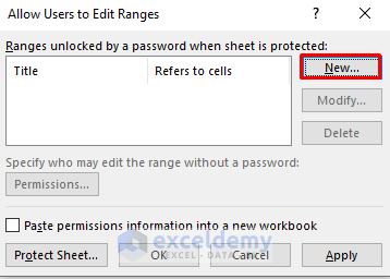
- First, go to the Review tab in the ribbon.
- Select Allow Edit Ranges from the Protect group.

- Allow Users to Edit Ranges dialog box will appear.
- Then, select New.
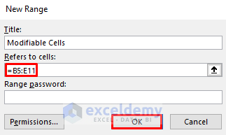
- After that, set the Title. Here, we set the title as Modifiable Cells.
- Set the Refers to Cells from cell B5 to cell E11.
- Click on OK.
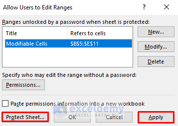
- Select the title and click on Apply.
- Next, select the Protect Sheet to protect cells except for those modifiable cells.
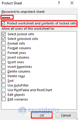
- A Protect Sheet dialog box will appear.
- Set any password in the password box.
- Check on the Protect worksheet and contents of locked cells.
- A Confirm Password dialog box will appear.
- Rewrite your given password.
- Click on OK.
- Next, try to alter any cells other than modifiable cells, and you will find the following result. See the screenshot.
Read More: How to Protect Excel Cells with Formulas
6. Embedding VBA Code to Protect Excel Cells from Being Edited
Finally, you can protect your Excel cells by utilizing VBA code. VBA code will help to protect excel cells without using the Protect Sheet. Here, in our dataset, we need to protect column F, column G, and column H. To apply the VBA code to protect Excel cells from being edited, you have to follow the following steps carefully.
Steps
- Press Alt+F11 to open the Developer tab. You can open it by customizing the ribbon.
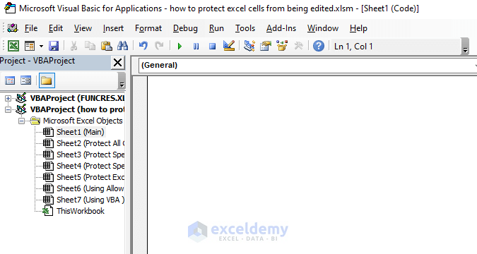
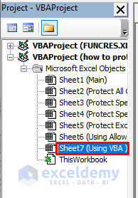
- Next, go to Sheet 7 from the Microsoft Excel Objects.
- A blank Editor box will appear.
- Then, write down the following code in the blank editor box.
Private Sub Worksheet_SelectionChange(ByVal Target As Range)

Dim i As Integer

    If Target.Column = 6 Then
    For i = 5 To 11
        If Target.Row = i Then
        Beep
        Cells(Target.Row, Target.Column).Offset(0, 1).Select
        End If
    Next i
    End If

    If Target.Column = 7 Then
    For i = 5 To 11
        If Target.Row = i Then
        Beep
        Cells(Target.Row, Target.Column).Offset(0, 1).Select
        End If
    Next i
    End If

     If Target.Column = 8 Then
    For i = 5 To 11
        If Target.Row = i Then
        Beep
        Cells(Target.Row, Target.Column).Offset(0, 1).Select
        End If
    Next i
    End If

End Sub- Now, close the Visual Basic window.
- Finally, you can see that you can’t select any cell in the range of cells F5:H11. That means your cells are protected.
Download Practice Workbook
Download the practice workbook
Conclusion
We have discussed 6 different methods to protect Excel cells from being edited. All the methods are fairly easy to use and very effective. If you have any questions, feel free to ask in the comment box.
Related Articles
- How to Unlock Cells without Password in Excel
- How to Protect Cells without Protecting Sheet in Excel
- Protect Excel Cells But Allow Data Entry
- How to Lock Cell Value Once Calculated in Excel
- How to Protect Excel Cells from Deletion
<< Go Back to Protect Excel Cells | Excel Protect | Learn Excel
Get FREE Advanced Excel Exercises with Solutions!
