Method 1 – Assigning a Dollar Sign ($) Manually to Cell References
Steps:
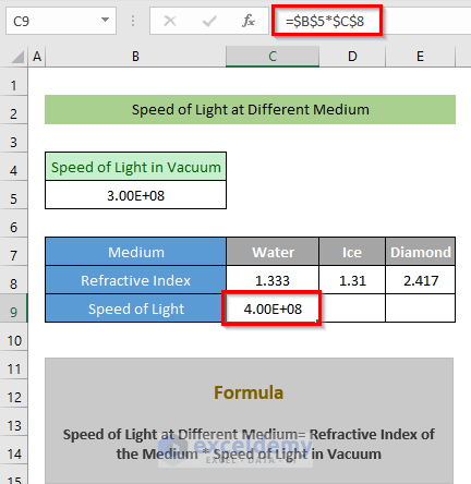
- Let’s calculate the speed of light for the Water medium.
- Select cell C9 to store the calculated value.
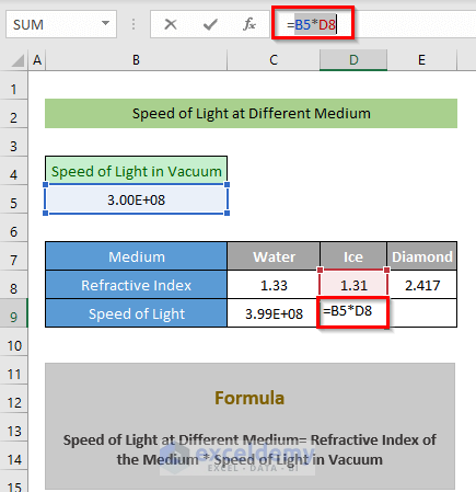
- Insert the following formula:
=B5*C8- These are now relative cell references.

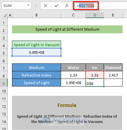
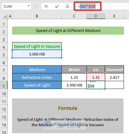
- Add Dollar Signs ($) before all the row and column numbers like this:
=$B$5*$C$8- Hit Enter.
Read More: How to Lock Certain Cells in Excel
Method 2 – Using the F4 Hotkey
- Select a cell to store the calculated value.
- Insert an equals sign.
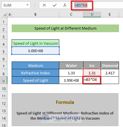
- Insert a formula and a cell reference.
- Click on the cell reference you need to lock.
- Press F4.
- Continue with the formula.
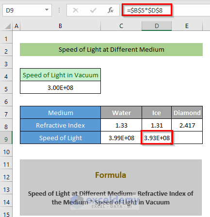
- Whenever you’re typing in a cell reference, press F4 to lock it.
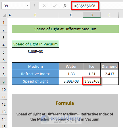
- Hit Enter.
Read More: Protect Excel Cells But Allow Data Entry
Additional Tips
You can toggle between Relative, Absolute, and Mixed cell references by pressing the F4 hotkey.
Part 1 – Toggle from Relative to Absolute Cell Reference
- Select the Cell Reference in the Formula Bar.
- Press the F4 key.
Part 2 – Toggle from Absolute to Relative Cell Reference
- Press the F4 key. The row numbers are locked up now.
- Press the F4 key again to lock the column number from the row number.
Part 3 – Toggle back to Relative Cell Reference
- Press the F4 key once again.
Things to Remember
- Assign a Dollar Sign ($) before the row and the column number to lock a cell.
- Use the F4 hotkey to lock a cell instantly.
- Pressing F4 cycles between the four possible cell reference options: relative > absolute > locked row > locked column > relative.
Download the Practice Workbook
Related Articles
- How to Lock Multiple Cells in Excel
- How to Protect Excel Cells with Formulas
- How to Protect Excel Cells with Password
- How to Protect Excel Cells from Deletion
- How to Protect Cells Without Protecting Sheet in Excel
- How to Lock Cell Value Once Calculated in Excel
- How to Unlock Cells without Password in Excel
<< Go Back to Protect Excel Cells | Excel Protect | Learn Excel
Get FREE Advanced Excel Exercises with Solutions!
