In this article, I will show you a variance formula that can show results with plus and minus signs in Excel. Variance is a mathematical term that denotes how much data disperse from the mean. Variance also can mean the difference between the actual and budgeted amounts. When you mean the first one mentioned here, you should know that variance can have no negative values. Because, you first get the differences between the mean and actual data, square the differences, and then sum them up. Then you divide the result by the number of data and get variance (also known as σ2).
But to know the positive and negative variations of actual data from forecast data, you may need to have simple variance formula that can show up plus and minus signs to display the direction of variance. So, let’s dive into the main discussion.
What Is Variance Formula?
Mathematically, variance is denoted by σ2, where
x = mean
xi= each data
i=1,2,3,4,….,i.e. number of data points
For example, if you have some numbers, 1,2,3,4,5 in one set and 1,2,1,2,5 in another set.
1st mean, x1=(1+2+3+4+5)/5=3
2nd mean x2=(1+2+1+2+5)/5=2.2
Then the variances of the two sets are,
σ12=[(1-3)2+(2-3)2+(3-3)2+(4-3)2+(5-3)2]/5=(4+1+0+1+4)/5=2
And, σ22=[(1-2.2)2+(2-2.2)2+(1-2.2)2+(2-2.2)2+(5-2.2)2]/5=10.8/5=2.16
This means the second set of data is more dispersed than the first one.
But wait.
If you have business data where some actual and forecast values are given, this variance formula is of use not anymore!
Because now you are not meant to find the average of the data to show the deviation from it. You just need to calculate the difference between the actual and budgeted values. A few simple calculations, right?
Well, that’s true. The formula will be just simple as the following this time:
This is the basic formula, depending on which value is greater, actual or forecast, this formula will show results with plus and minus signs. In the next section, we will see an example to use this formula in Excel more meaningfully.
How to Apply Variance Formula in Excel and Get Plus-Minus Results: with Easy Steps
In this example, we will show the application of the variance formula with positive and negative results. Here, we have a dataset of the projected and actual profit of an organization. We will apply the variance formula to this dataset. Then we will create a variance chart too.

📌 Step 1: Apply Variance Formula to Calculate Difference Between Actual and Forecast Values
First, we will calculate the variance.
- Go to Cell E5 and put the following formula in it.
=D5-C5
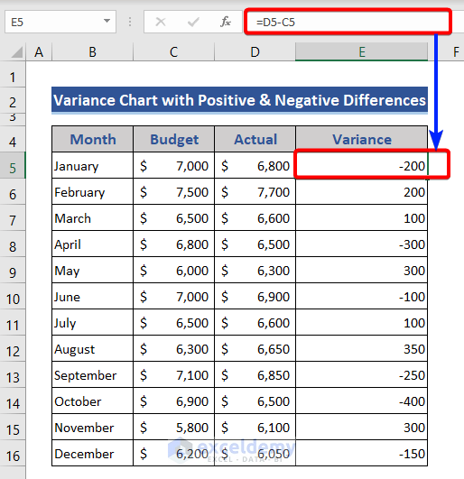
We get the variance with the plus and minus symbols.
Read More: How to Do Variance Analysis in Excel
📌 Step 2: Separate the Negative and Positive Differences into Two Columns
Now, we will separate the negative and positive values. We will do this using the IF function.
- Go to Cell F5 and Write the following formula.
=IF(E5<0,E5,"")
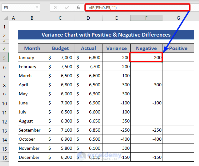
We separate the negative values.
- After that, we go to Cell G5 and put the below formula.
=IF(E5>0,E5,"")

Thus, we separate the positive and negative values.
Read More: How to Calculate Sample Variance in Excel
📌 Step 3: Choose a Suitable Symbol to Create a Chart
Now, we will choose a symbol to present the chart. We will place the symbol in a remote cell to avoid a mixture with the original data, here in Cell A18.
- Choose the Symbol option from the Symbols group of the Insert tab.

- The Symbols window appears.
- Choose Arial from the Font section, and Block Elements from the Subset section.
- After that, choose a symbol and finally click on the Insert tab.

- We can see a symbol has been added to the dataset.

Read More: How to Find Population Variance in Excel
📌 Step 4: Add Custom Repetition to the Symbol for Each Variance with REPT Function
Now, we will form a chart combining the symbol and values with the combination of the IF, REPT, and ABS functions.
- Go to Cell H5 and put this formula.
=IF(F5="","",F5&" "&REPT($A$18,ABS(F5)/100))
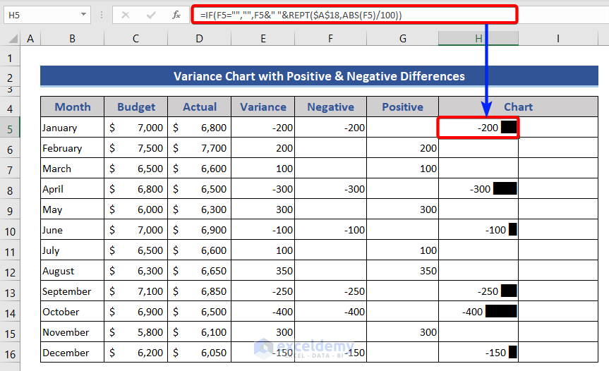
We can see a chart for negative values is showing in the dataset.
- Similarly, we put this formula for the positive values on Cell I5.
=IF(G5="","",REPT($A$18,ABS(G5)/100)&" "&G5)

- Now, we choose the color and alignment from the Font and Alignment group.

Read More: How to Find the Variance of a Probability Distribution in Excel
Download Practice Workbook
Download this practice workbook to exercise while you are reading this article.
Conclusion
In this article, we described an example to explain the application of the variance formula in excel with plus-minus results. I hope this will satisfy your needs. Please give your suggestions in the comment box.
Related Articles
- How to Calculate Percentage Variance between Two Numbers in Excel
- How to Calculate Pooled Variance in Excel
- How to Calculate Coefficient of Variance in Excel
- How to Calculate Mean Variance and Standard Deviation in Excel
<< Go Back to Calculate Variance in Excel | Excel for Statistics | Learn Excel
Get FREE Advanced Excel Exercises with Solutions!
