How to Calculate Percentage Variance Between Two Numbers in Excel

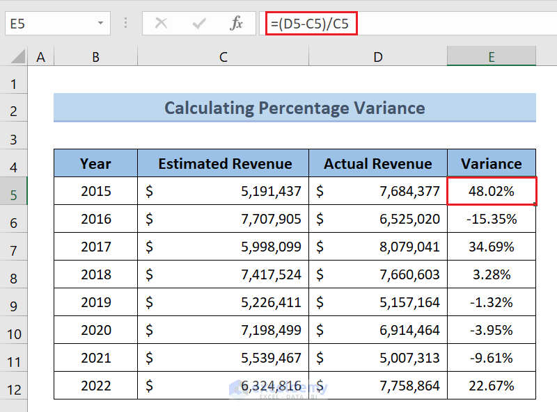
The following dataset illustrates how to calculate the percentage variance between values in the Estimated Revenue and Actual Revenue columns. The Variance column shows the percentage change for each year.

Method 1 – Combining Simple Formula & ABS Function

Steps:

• Select the output column > Home tab > Number group > Number Format drop-down > Percentage.
  
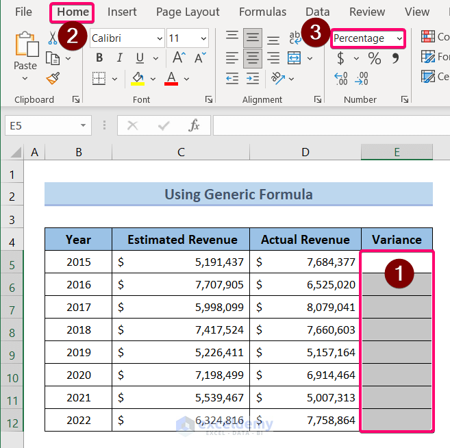
• Select a blank cell.
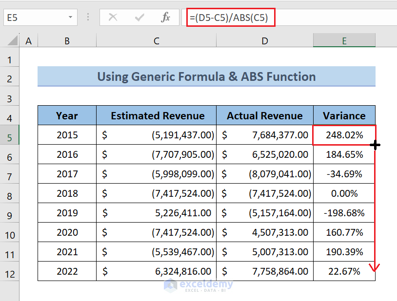
• Enter the formula: =(D5-C5)/ABS(C5)
• Replace C5 and D5 with your initial value and final value.
• Press Enter.
  Note: If you want the absolute value of percentage variance, use: =ABS((D5-C5)/C5)Drag the Fill Handle down the column.
  The column will be filled with percentage variance accordingly.
  Note: You can change the number of decimal places from the Home tab > Number group > Decrease Decimal/Increase Decimal option.

Method 2 – Using Arithmetic Formula

Steps:

• Select the output column > Home tab > Number group > Number Format drop-down > Percentage.
• Select a blank cell.
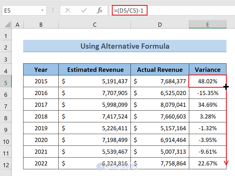
• Enter the formula: =(D5/C5)-1
  Replace C5 and D5 with your initial value and final value.
• Press Enter.
• Use the Fill Handle to copy the formula down the column.

The percentage changes will be calculated accordingly.

Handling #DIV/0! Error While Calculating Percentage Variance Between Two Numbers in Excel

A division process is involved in calculating the percentage change between two values. If the denominator is 0, Excel will show a #DIV/0! error. The nested IF function, along with the IFERROR function, is used to tackle this error. Here’s how:

• Select your output cell.
• Insert the formula: =IF(D5<>0, IFERROR((D5-C5)/C5, 1), IFERROR((D5-C5)/C5, 0))
• Replace C5 and D5 with your initial value and final value.
• Press Enter.

The error will be tackled to show the percentage change.
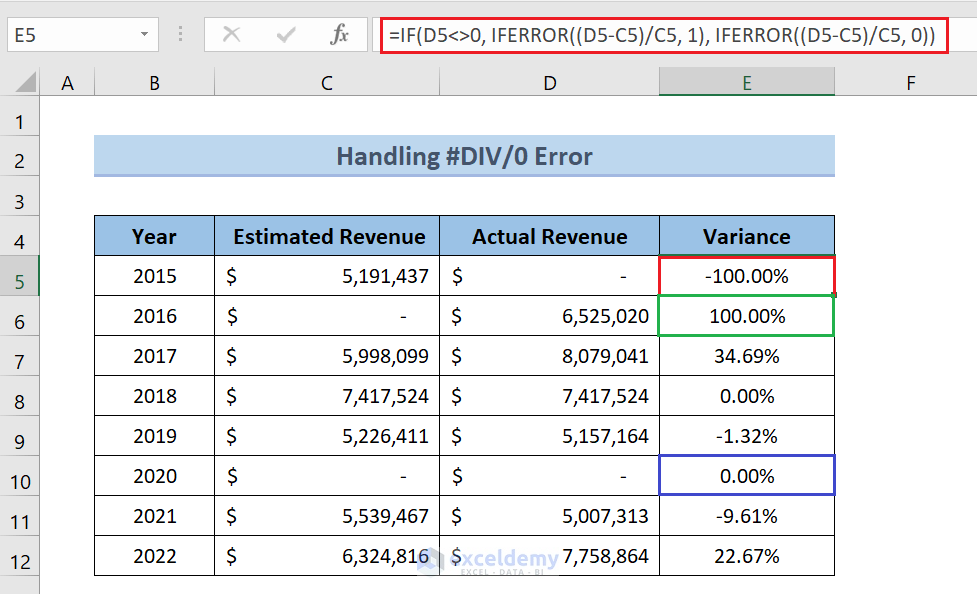Note: When both the values are 0, the percentage change will be considered 0%. If the initial value is 0 but the final value is not, the percentage change will be considered 100%.

Download the Practice Workbook

You can download the Excel file and practice.

<< Go Back to Calculate Variance in Excel | Excel for Statistics | Learn Excel