Step 1 – Calculating Total Quantities Sold
- Select the C11 cell and use the following formula:
=SUM(C5:C10)- Hit Enter.
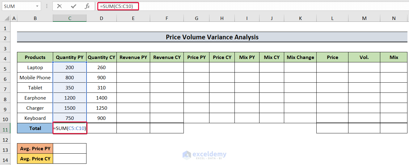
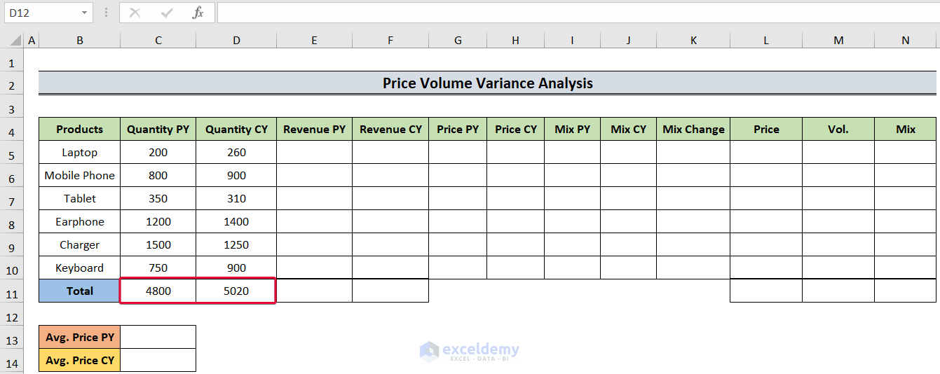
- We will have the sum of the goods sold for the previous year.
- Select the D11 cell and use the formula below:
=SUM(D5:D10)- Hit Enter.
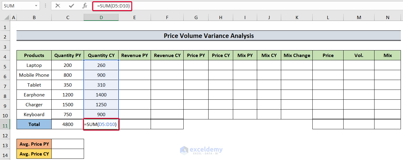
- We will get the quantity sold for the current year.
Read More: How to Calculate Variance of Stock Returns in Excel
Step 2 – Determining the Total Revenue
- Firstly, choose the E11 cell and use the following:
=SUM(E5:E10)- Press Enter.
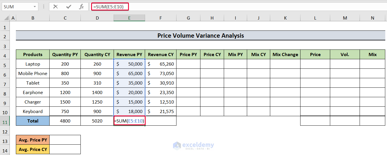
- We will get the total revenue for the past year.
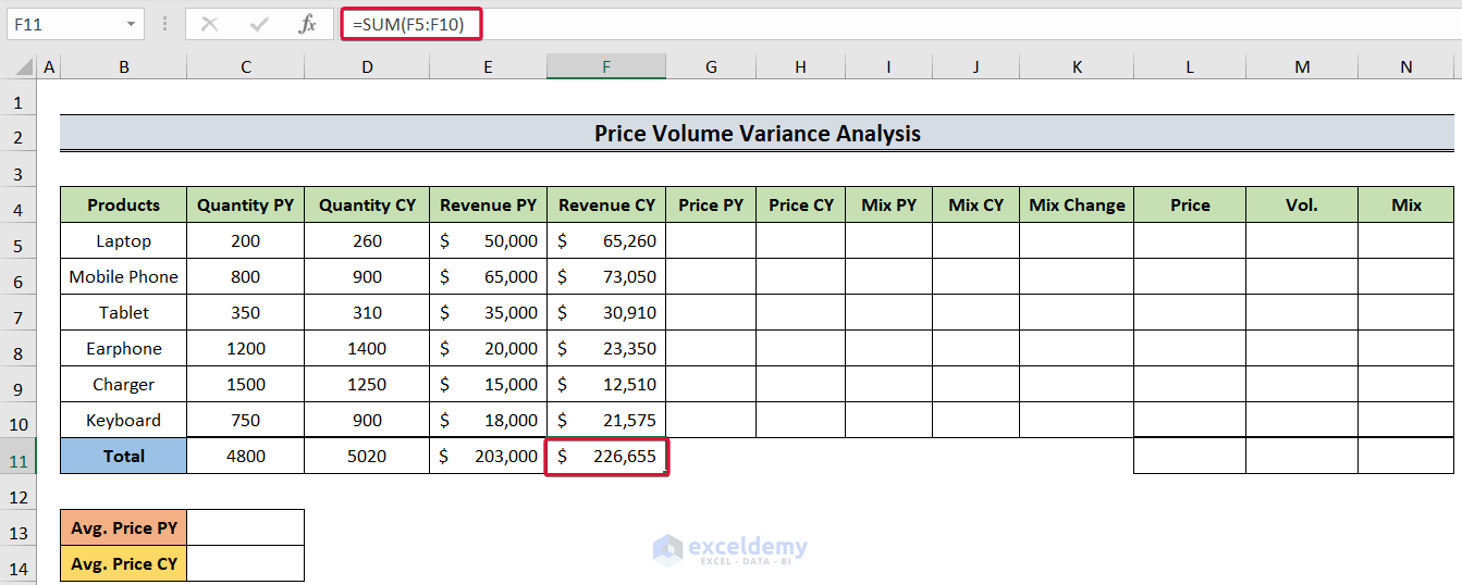
- Select the F11 cell and use:
=SUM(F5:F10)- Hit Enter to get the total revenue for this year.
Read More: How to Create Minimum Variance Portfolio in Excel
Step 3 – Evaluating Revenue Per Unit
Revenue Per Unit = Revenue of the product / Unit sold of that product
- Choose the G5 cell and enter the following formula:
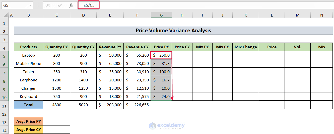
=E5/C5- Hit Enter.
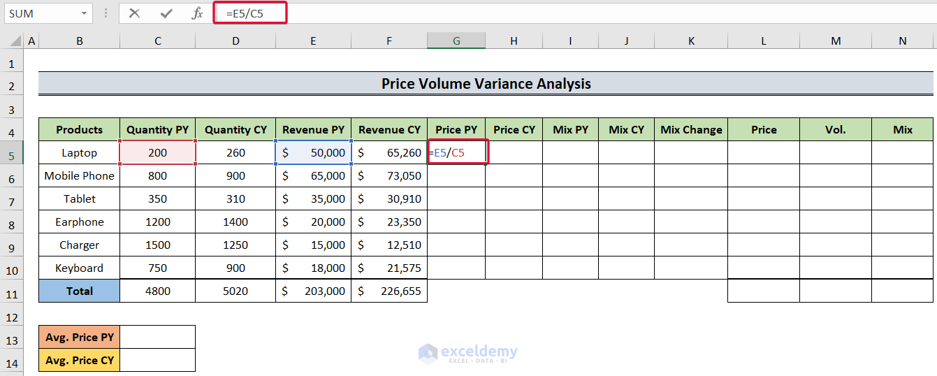
- We will have the price for the first product.
- Lower the cursor down to autofill the answers.
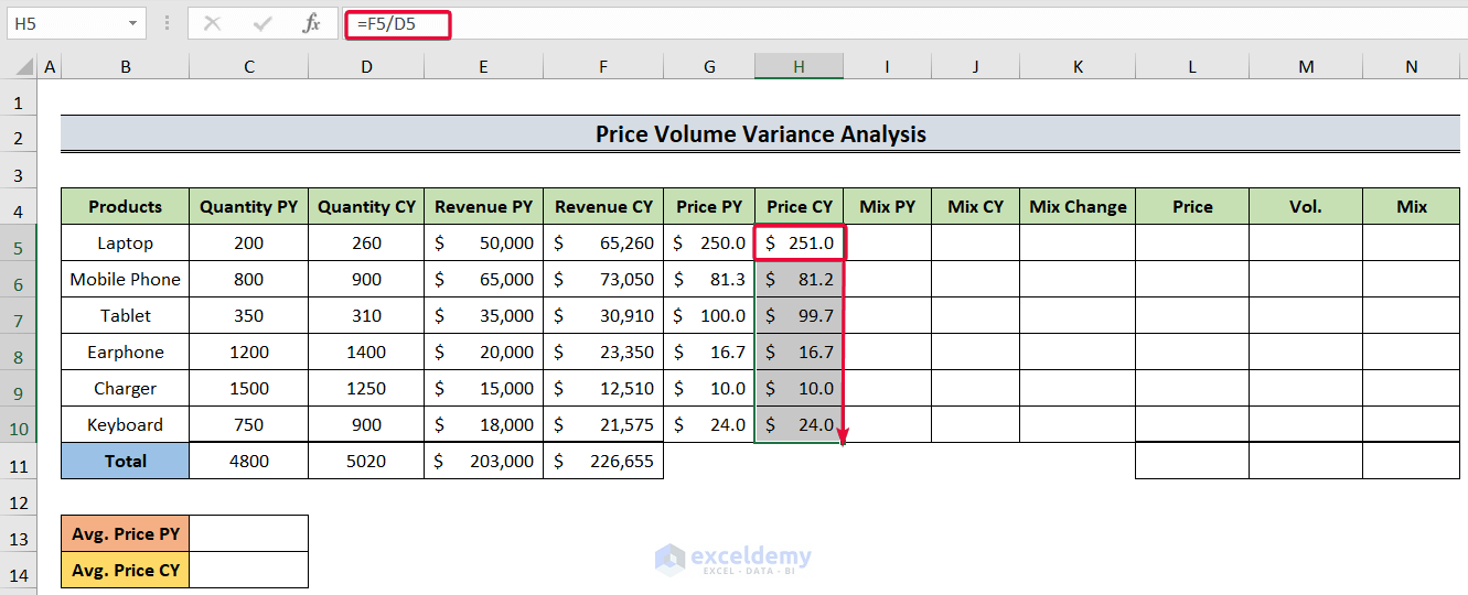
- Click on the H5 cell and use:
=F5/D5- Hit the Enter button.
- We will get the price for the current year.
- Move the cursor down to the last cell to autofill the cells.
Read More: How to Calculate Schedule Variance Using Excel Formula
Step 4 – Calculating the Average Price
Average Price = Total revenue / Total quantities sold
- Select the C13 cell and enter the following:
=E11/C11- Hit the Enter button.
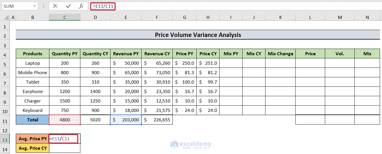
- We will get the average price for the last year.
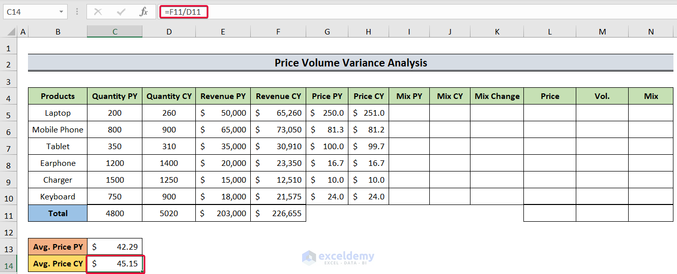
- Select the C14 cell and enter:
=F11/D11- Hit Enter to get the average price for the current year.
Read More: Budget vs Actual Variance Formula in Excel
Step 5 – Determining the Mix
Mix is the percentage of a particular good sold in total goods sold.
Mix = (Quantities of a particular good sold / Total goods sold) * 100
- Choose the I5 cell and insert the following:
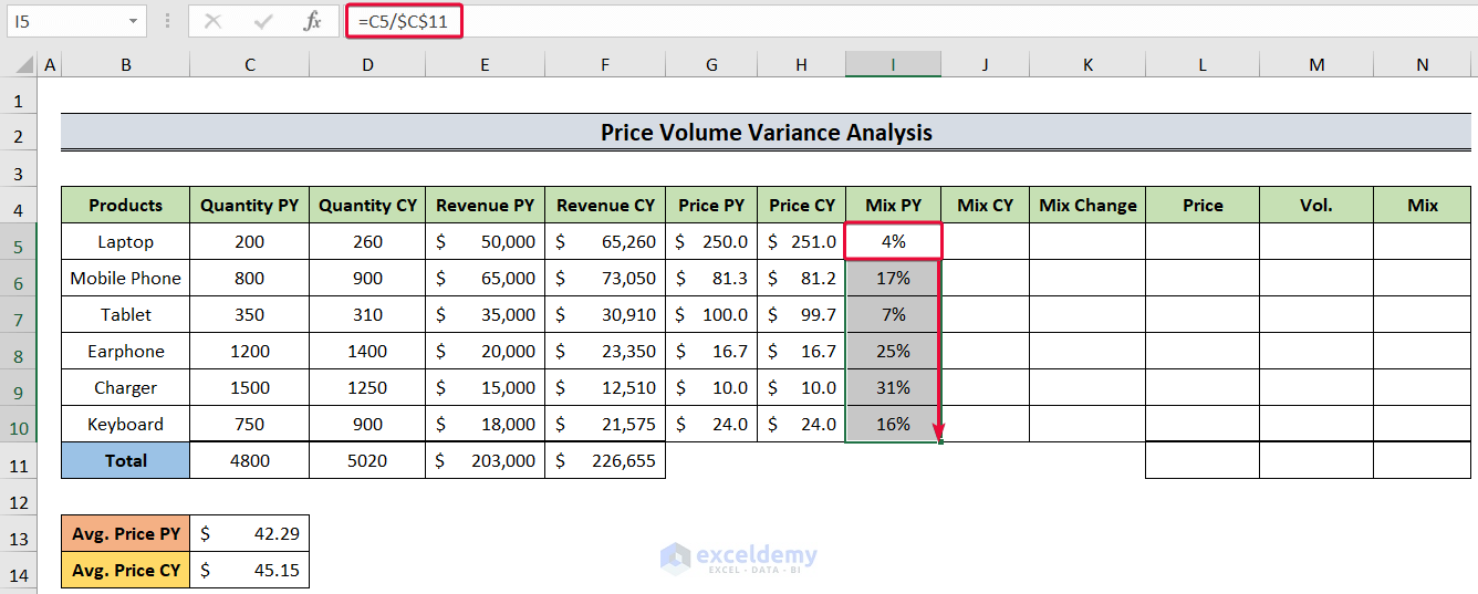
=C5/$C$11- Press Enter.
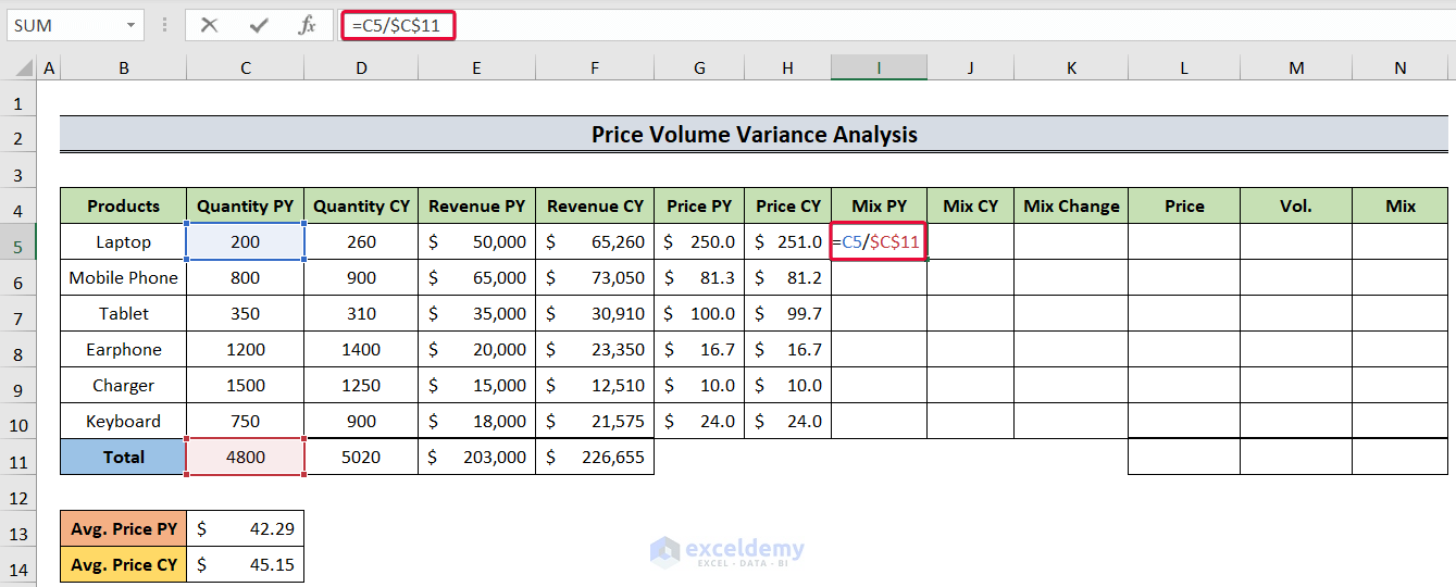
- We will have the mix for that year.
- Move the cursor down to the last cell to autofill.
- Repeat the same process for the current year with the formula in the J5 cell being:
=D5/$D$11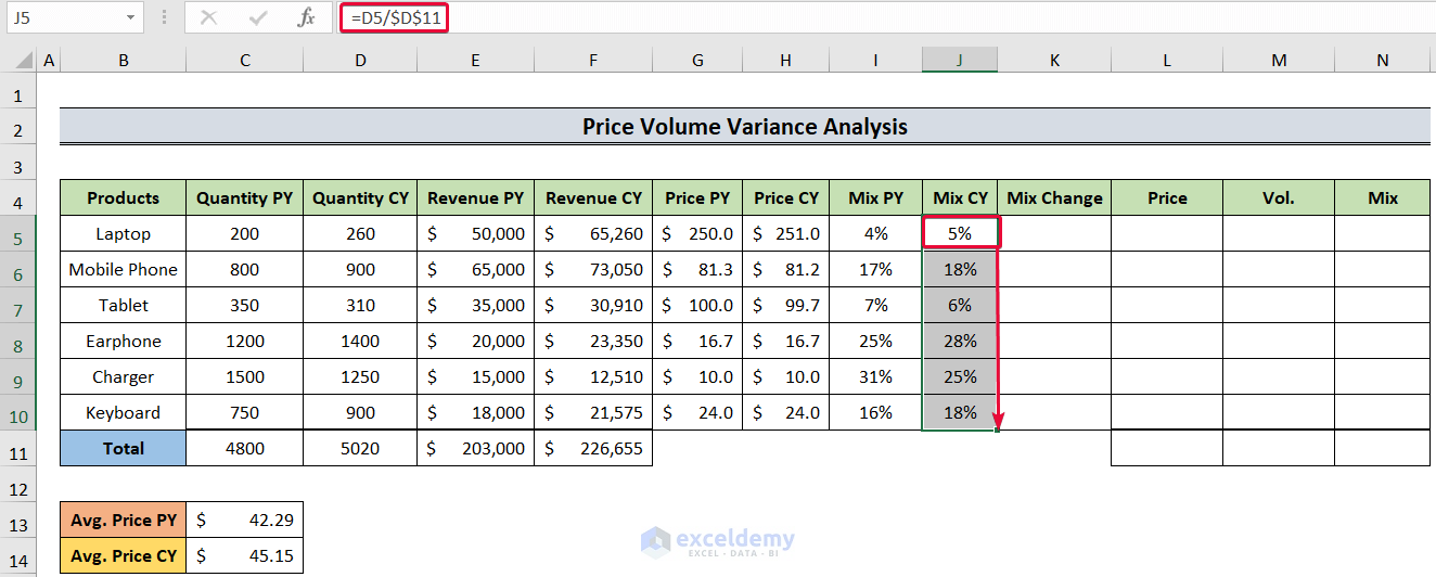
Read More: How to Calculate Portfolio Variance in Excel
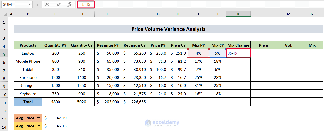
Step 6 – Calculating the Mix Change
Mix Change = Mix of current year- Mix of the previous year
- Select the K5 cell and use:
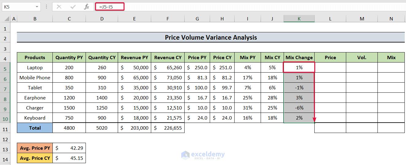
=J5-I5- Hit Enter.
- We will get the differences in mix.
- Drag the cursor down to autofill the cells.
Read More: How to Calculate Budget Variance in Excel
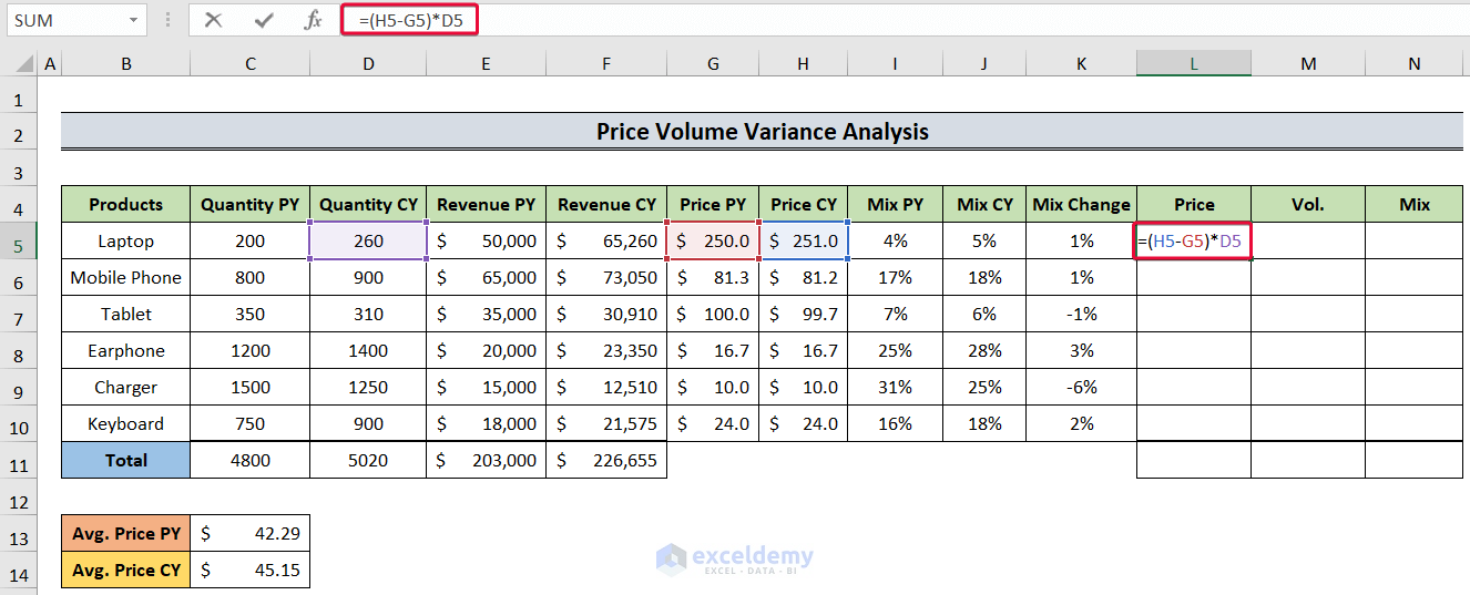
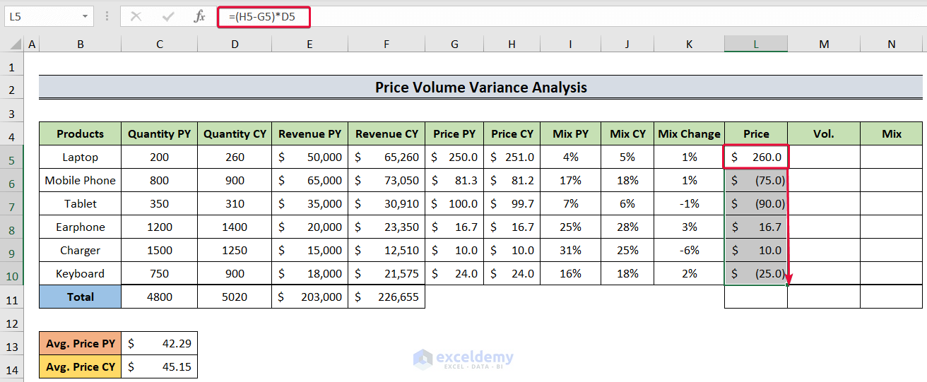
Step 7 – Evaluating the Price Variance
Price Variance = (Price CY – Price PY) * Quantity CY
- Select the L5 cell and insert the following:
=(H5-G5)*D5- Hit Enter.
- We will get the price variance for that product.
- Drag the cursor down to the L10 cell to autofill.
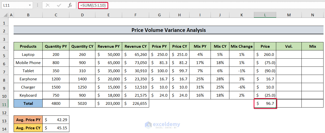
- Select the L11 cell and enter the following:
=SUM(L5:L10)- Press the Enter button.
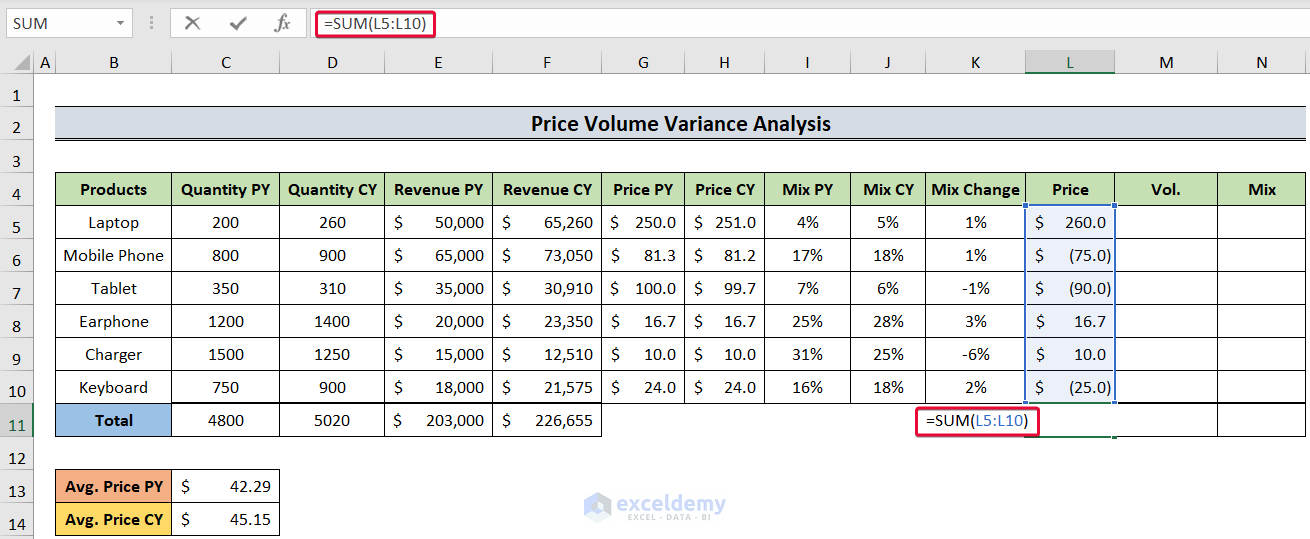
- We will get the sum of the products’ price variances.
Read More: How to Calculate Variance Inflation Factor in Excel
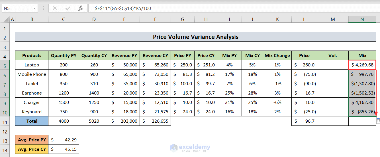
Step 8 – Determining the Mix Variance
Mix Variance = Revenue PY * (Price PY – Average Price PY) * Mix Change/100
- Select the N5 cell and enter the following formula:
=$E$11*(G5-$C$13)*K5/100- Hit Enter.
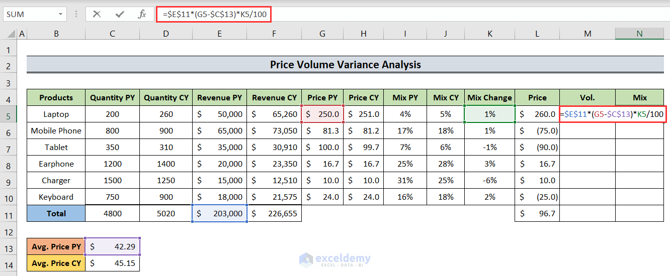
- As a result, we will get the mic variance for that product.
- Move the cursor to the N10 cell to autofill the rest of the cells.
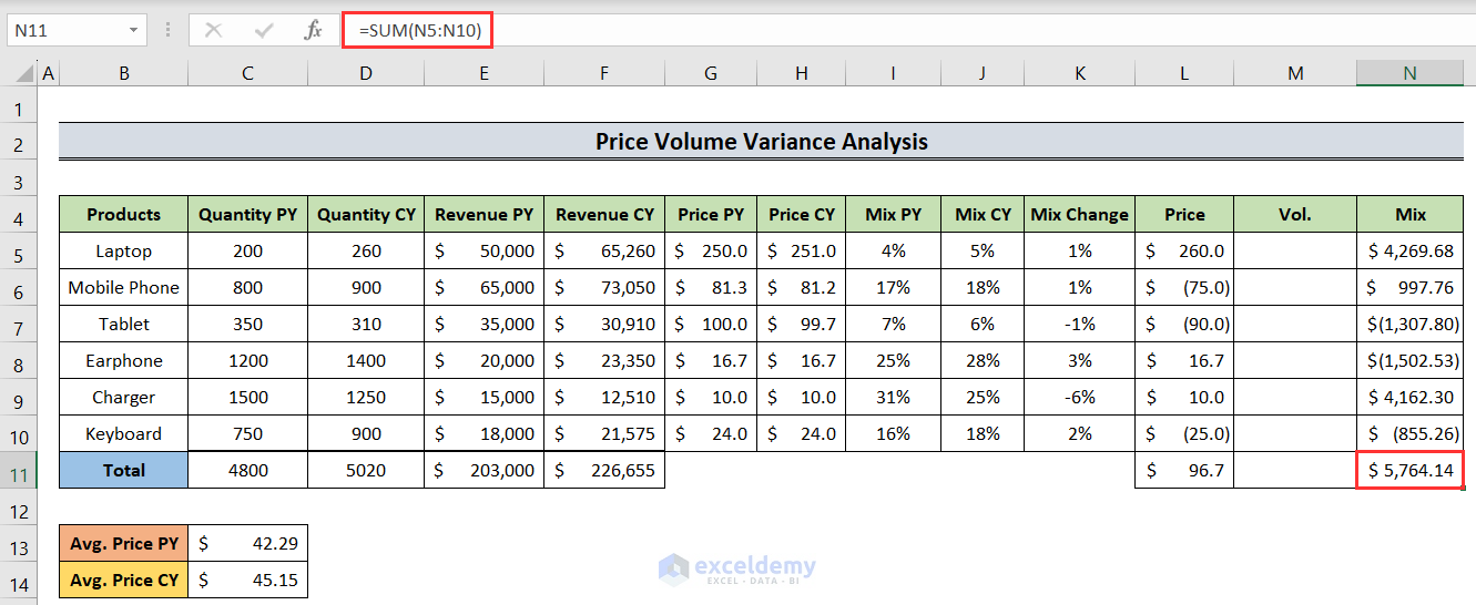
- Select the N11 cell and insert the following:
=SUM(N5:N10)- Hit the Enter button.
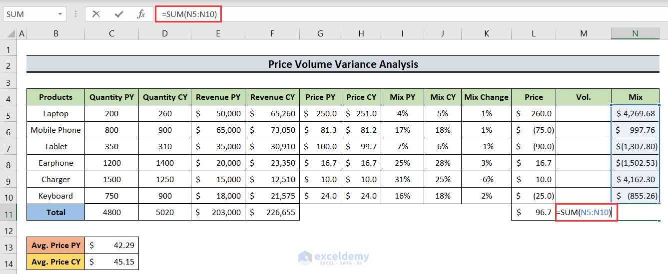
- As a result, we will have the sum of all mix variances. It is too a positive number which means a favorable one.
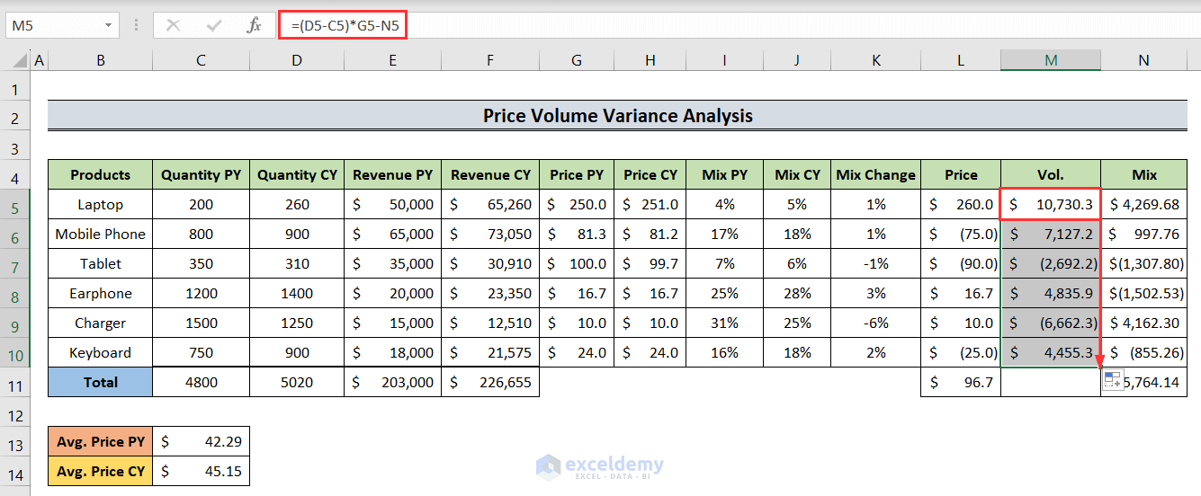
Step 9 – Calculating Volume Variance
Volume Variance = (Quantity CY – Quantity PY) * Price PY – Mix Variance
- Select the M5 cell and insert:
=(D5-C5)*G5-N5- Press the Enter button.
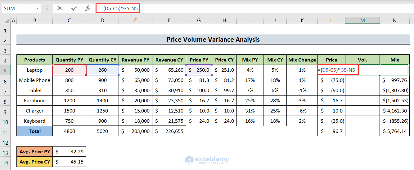
- We will get the volume variance for that product.
- Drag the cursor down to the M10 cell to autofill the values.
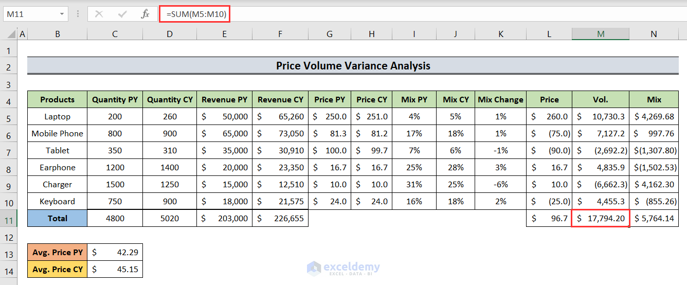
- Select the M11 cell and input the following:
=SUM(M5:M10)- Hit Enter.
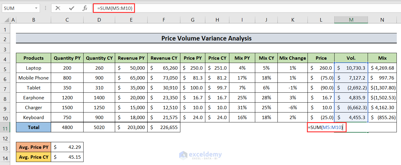
- We will get our volume variance.
Result Interpretation:
The values with bracket represent negative values.
Here’s how to understand what they mean:
1. Price Variance: This shows how much the change in prices affected the total revenue. If it’s positive, it means the price increase helped make more money. If it’s negative, the price decrease hurts the revenue. In the dataset above, the Total Price Variance is $96.7. It depicts that the owner is capable of making more money.
2. Volume Variance: This tells us how much the change in the number of items sold affected the total revenue. If it’s positive, it means selling more items boosted the revenue. If it’s negative, selling fewer items lowered the revenue. In this case, the Total Volume Variance is also positive with a value of $17,794.20. This means the seller was selling more items than previous year.
3. Mixed Variance: Mix variance, also known as sales mix variance, reveals how the proportion of different products or services sold affected the revenue change. If it’s positive, it means the sales mix of products contributed favorably to the revenue change. If it’s negative, the sales mix had a less favorable impact on revenue. Here, the Total Mixed Variance seems also positive with a value of $5764.14. This defines that total mixed sales are responsible for overall revenue growth.
By doing this analysis, you can figure out what caused the revenue to change, whether it was because of price changes, selling more or fewer items, or both. It helps businesses understand how their sales are performing and make decisions on pricing and sales strategies accordingly.
Read More: How to Calculate Semi Variance in Excel
Download the Practice Workbook
<< Go Back to Calculate Variance in Excel | Excel for Statistics | Learn Excel
Get FREE Advanced Excel Exercises with Solutions!

Are there any detailed explanation on the mix variance formula?
Mix Variance = Revenue PY*(Price PY – Average Price PY)*Mix Change/100
I cannot figure out why we need to divide the formula by 100.
Thanks
Hello JC, thanks for reaching out. Here, the main formula for Mix Variance is:
Mix Variance = Revenue PY*(Price PY – Average Price PY)*(% of Mix CY – % of Mix PY). Although the Mix PY and CY were shown in percentage format in the article, we didn’t calculate these values as percentage. So in the formula, the difference of Mix CY and PY is divided by 100.
Can you explain in detail for the mix variance? I cannot figure out why we have to start with budgeted sales revenue and divide the whole formula by 100.
Mix Variance = Revenue PY*(Price PY – Average Price PY)*Mix Change/100
Hello Justin, thanks for reaching out. Here, the main formula for Mix Variance is:
Mix Variance = Revenue PY*(Price PY – Average Price PY)*(% of Mix CY – % of Mix PY). Although the Mix PY and CY were shown in percentage format in the article, we didn’t calculate these values as percentage. So in the formula, the difference of Mix CY and PY is divided by 100.
Thanks for the info. It’s confusing to include the division by 100 when most readers will not understand why it’s there. I would suggest removing it when you come to review the article. Thanks again.
Thanks David for your feedback. The formatting of Mix PY, Mix CY and Mix Change being in percentage made it a bit confusing. We’ll update it soon.
Hi, thanks for this. However in the formula for the mix variance, you used QTY CY rather than Revenue PY. Is this correct or an error? Please check again and confirm. Thank you
Hello Ayodeji Aboderin, thanks for reaching out. You are right, there was an error. Now, the article is updated accordingly. Please let us know if you have any other queries.
Regards
Sajid Ahmed
Exceldemy
Hello!
can you please update the conclusion and explain how to conclude the result, what it depicts and how to interpret the data? if possible?
thank you!
Also, the explanation for the steps is great! Helped a lot!
Hey there, Mr. Chhavi.
Thanks a lot for your feedback.
“Here’s how to understand what they mean:
1. Price Variance: This shows how much the change in prices affected the total revenue. If it’s positive, it means the price increase helped make more money. If it’s negative, the price decrease hurts the revenue.
2. Volume Variance: This tells us how much the change in the number of items sold affected the total revenue. If it’s positive, it means selling more items boosted the revenue. If it’s negative, selling fewer items lowered the revenue.
3. Mixed Variance: Mix variance, also known as sales mix variance, reveals how the proportion of different products or services sold affected the revenue change. If it’s positive, it means the sales mix of products contributed favorably to the revenue change. If it’s negative, the sales mix had a less favorable impact on revenue.
By doing this analysis, you can figure out what caused the revenue to change, whether it was because of price changes, selling more or fewer items, or both. It helps businesses understand how their sales are performing and make decisions on pricing and sales strategies accordingly.”
I hope you have your answer here. And sorry for the inconvenience. We would love to hear from you again.
Regards
ExcelDemy Team
The formulas in the Excel download file for Mix is different than the screenshots in the article. Can you explain the difference? One uses current year quantity and the other uses prior year revenue.
Excel File=$D$11*(G5-$C$13)*K5/100
Article above=$E$11*(G5-$C$13)*K5/100
please where i can get the file
Hello Nourhan Essam,
You can download the Excel file from the Download section.
Here, I’m also attaching the Excel file link: Analysis of Price Volume Variance.xlsx
Regards
ExcelDemy
Hello JOHN C,
Yes, you are right, the formula for calculating the Mix value is different in the given Excel file and the above article.
The formula mentioned in our article is correct. There must have been an error while selecting cell E11, hence the adjacent cell D11 is present in the Excel file formula.
We have updated the Excel file with the correct formula. Thanks for your feedback.
Regards,
Seemanto Saha
Exceldemy
Hello,
Thank you for this guide.
I was wondering how you would change these calculations for products that are new or are discontinued.
Thanks!
Hello Michiel,
Thanks for your question. If you want to add new products to the dataset and include them in your calculation, you will have to convert the range into a table. Then you will be able to add as many new products as you required by inserting new rows in the dataset.
On the other hand, if the products in the dataset are discontinued, you don’t need to modify any cells that contain the “Quantity” or “Revenue” values since we are not doing any arithmetic operation on them. For safety reasons, you can apply the IFERROR()function in all the cells where you are applying formula. For example, you would change the formula in Column G into IFERROR(E5/C5). The exception is the cells where we will calculate the sum of different values. For those cells, we will modify the formula of M11 into SUM(IF(ISNUMBER(M5:M10), M5:M10)).
Hopefully, you have got the desired answer.
Why is the Mix variance based on REVENUE PY* and not QUANTITY PY?
Mix Variance old = Revenue PY*(Price PY – Average Price PY)*Mix Change/100
Mix Variance new = Quantity PY*(Price PY – Average Price PY)*Mix Change/100
Hi Strike,
Thanks for your comment. The Mix Variance formula provided in the article is based on Revenue rather than Quantity because it is intended to capture the impact of changes in the sales mix of different products on revenue, which includes both price and quantity components. Here’s the formula:
Mix Variance = Revenue PY * (Price PY – Average Price PY) * Mix Change / 100
By using Revenue PY in the formula, you are considering both the price and quantity component. Thus it becomes a comprehensive way to evaluate how the mix of products contributed to changes in revenue. It provides a more complete picture of why the revenue changed. Using Quantity alone would only consider the quantity component and not account for price changes, which are also crucial in understanding revenue variations.
If you have any further query, then please inform us in the reply section.
Regards,
ExcelDemy Team
Why is the Volume Variance based on the prior year price, but the Price Variance is based on the current year volume?
Hi KIEL,
Thanks for your question. Actually, you may seem that the choice of using prior year prices for Volume Variance and current year volumes for Price Variance is wrong, but it aligns with certain assumptions and conventions often used in variance analysis. Let me explain the reasoning behind this choice:
1. Volume Variance based on Prior Year Price:
The assumption here is that changes in quantities sold are evaluated against the prices of the prior year. Volume Variance assesses the impact of selling more or fewer units than planned at the prior year’s prices. Using the prior year’s price isolates the impact of changes in quantity sold, assuming that the pricing structure from the prior year remains relevant.
2. Price Variance based on Current Year Volume:
Here, we’re checking how price changes between this year and last year affect earnings, considering the amount sold this year. We assume that this year’s sales volume reflects the current business situation, and any price changes are looked at based on this year’s sales.
I think you have understood the matter. If you have any further queries please inform us in the reply.
Warm Regards,
ExcelDemy Team