How to Calculate Variance Inflation Factor in Excel

In this article, we will learn to calculate the variance inflation factor in Excel. It is also expressed as VIF. Variance Inflation Factor or VIF detects the severity of multicollinearity in regression analysis. Today, we will show step-by-step procedures. Using these steps, you can easily calculate the variance inflation factor in Excel.

What Is Variance Inflation Factor (VIF)?

Multicollinearity in regression analysis is seen when two or more variables are strongly correlated. Because of the strong correlation, they do not provide any unique or independent information in the regression model. If the correlation among variables is high, then it causes problems fitting and interpreting the regression model.

To detect the multicollinearity, we use the variance inflation factor or VIF. The VIF determines the severity of the correlation between explanatory variables in a regression model. After determining the VIF for each explanatory variable, we can decide if multicollinearity can cause problems for the model or not.

The general form of the equation for calculating VIF is:

=1/(1-R²)

Here, R² is known as the R-squared value.

How to Calculate Variance Inflation Factor in Excel: Step-by-Step Procedures

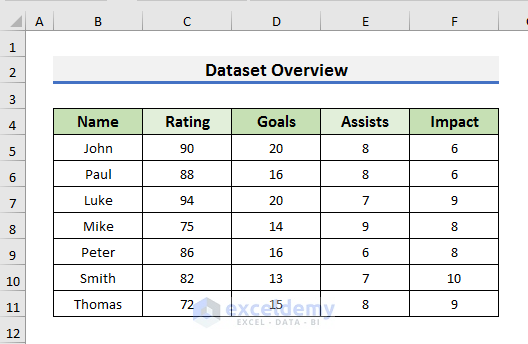
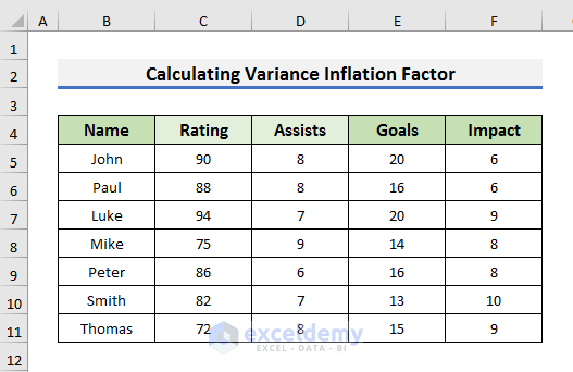
To explain the steps, we will use a dataset that contains the Rating, Goals, Assists, and Impact of some football players. Here, the Rating depends on the Goals, Assists, and Impact of a player. So, Rating is the response variable and others are explanatory variables. We will do regression analysis and find out the value of the Variance Inflation Factor for the explanatory variables. So, without further delay, let’s start the discussion.

STEP 1: Load Data Analysis ToolPak

First of all, we need to load the Data Analysis ToolPak.
To do so, click on the File tab.

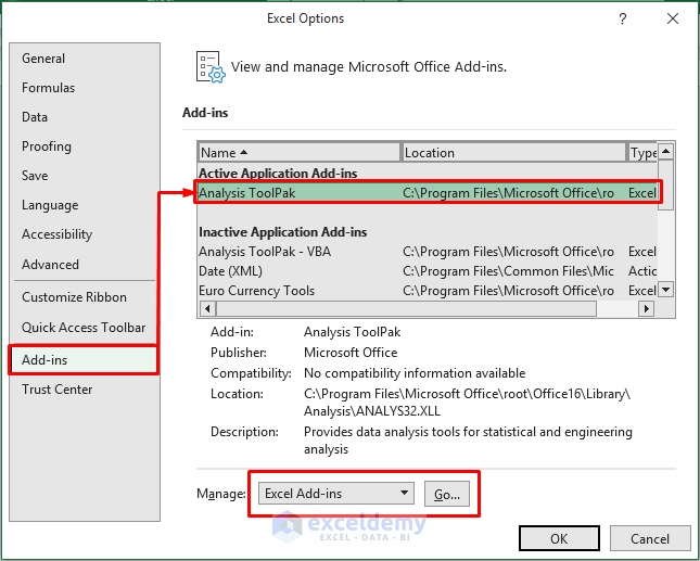
After that, select Options from the bottom left corner of the screen. It will open the Excel Options window.

In the Excel Options window, go to the Add-ins section first.
Then, select Analysis ToolPak.
After that, select Excel Add-ins in the Manage box and click on the Go option. It will open the Add-ins box.

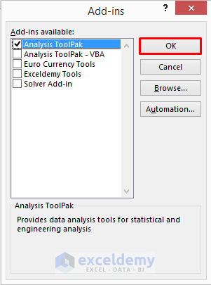
In the Add-ins box, check Analysis ToolPak.
Click OK to proceed.

STEP 2: Use Data Analysis Tool for Regression

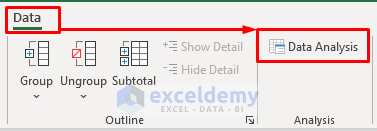
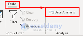
Secondly, go to the Data tab and select the Data Analysis option.

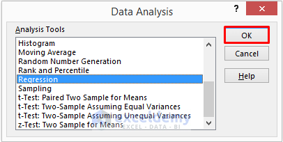
In the Data Analysis box, select Regression and click OK to proceed.

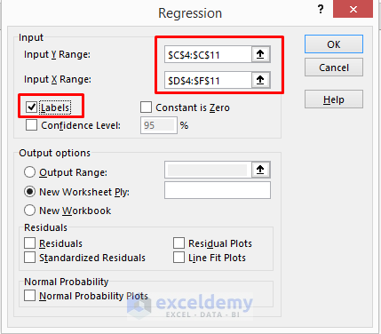
After that, you need to select the Input Y and X Ranges.
In Y Range, you need to insert the response variable.
In our case, that is the Rating. So, we inserted $C$4:$C$11 inside the Input Y Range box.
For Input X Range, we insert the explanatory variables.
So, we have inserted $D$4:$F$11 inside the Input X Range box.
Also, check Labels.
Click OK to proceed.

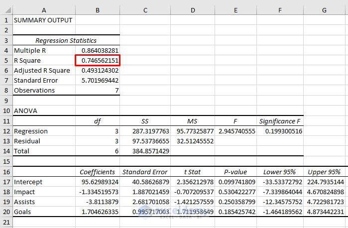
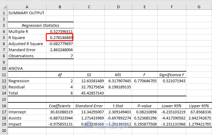
As a result, you will see the summary output in a new worksheet.
Check the R Square value from here.
The R Square value shows the strength of the relationship between the model and the explanatory variables.
Here, it is 0.75 or 75% which is good for a regression model.

STEP 3: Calculate VIF for Each Explanatory Variable

In the third step, go to the sheet that contains the dataset. Here, we will find the VIF for each explanatory variable.
For that purpose, we need to perform individual regression by using one explanatory variable as the response variable and the other two as the explanatory variable.
So, again go to the Data tab and click on the Data Analysis option.

In the Data Analysis box, select Regression and click OK to proceed.

In the Regression box, you need to select the Input Y and X Ranges.
Now, click on the Input Y Range box and enable editing.
Then, select the range $D$4:$D$11. Here, the “Goals” is the response variable and the Assists and Impact are the explanatory variables.
Next, click on the Input X Range box and select the range $E$4:$F$11.
Also, check Labels.
Click OK to proceed.

As a result, you will see the summary output in a new worksheet.
Note the R Square Because we need it to calculate the VIF of Goals.

After that, select Cell D5 and type the formula below:

=1/(1-B5^2)

Press Enter to see the VIF for Goals.

STEP 4: Determine VIF for Second Explanatory Variable

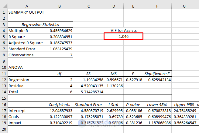
After finding the VIF for the first explanatory variable which is Goals, we need to find the VIF for Assists.
To do so, we need to make a change in the dataset.
Swap the position of the Assists column with the Goals column because you need a continuous range for Regression Analysis.

Now, follow STEP 3 to get the VIF for Assists.

STEP 5: Determine VIF for Third Explanatory Variable

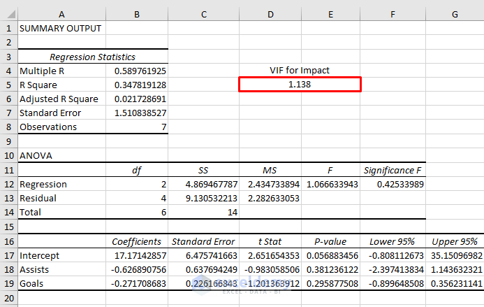
To find the VIF for Impact which is the third explanatory variable, keep the Impact column in Column D and the others in Columns E and F.

After that, follow STEP 3 to find the VIF for Impact.
You can follow the same steps if you have more variables.
You can see the VIF for Impact is 1.138.

STEP 6: Analyze Variance Inflation Factor or VIF

The value of VIF shows how strong the correlation between the variables is.
If the VIF is 1, then, there is no correlation.
If it is between 1 to 5, then there is a moderate correlation that doesn’t affect the regression model.
If the VIF is greater than 5, then there is a strong correlation between the variables and it needs attention.
In our case, the VIF values for Goals, Assists, and Impact are close to 1.
So, we can say multicollinearity is not a problem for our regression model.

Read More:

Download Practice Workbook

You can download the workbook from here.

Variance Inflation Factor.xlsx

Conclusion

In this article, we have demonstrated step-by-step procedures to calculate Variance Inflation Factor in Excel. I hope this article will help you to perform your tasks efficiently. Furthermore, we have also added the practice book at the beginning of the article. To test your skills, you can download it to exercise. Lastly, if you have any suggestions or queries, feel free to ask in the comment section below.

<< Go Back to Calculate Variance in Excel | Excel for Statistics | Learn Excel

Get FREE Advanced Excel Exercises with Solutions!

2 Comments

Sarah Apr 17, 2023 at 3:31 PM

Hi and thanks for this article !

I have a question, how can we interpret a VIF where the R square is 1 ?
The formula would be : 1 / (1-1) so 1/0 which is impossible…
I have this issue with some variables…

Can you help me ?

Thank you again !
- Reply
  Mursalin Ibne Salehin Apr 18, 2023 at 12:06 PM
  
  Dear SARAH,
  Thanks for your comment. The Variance Inflation Factor (VIF) measures the degree of multicollinearity in a set of explanatory variables in a regression model. VIF values greater than 1 indicate that the explanatory variables are correlated to some degree. However, a VIF value of infinity is not an indication of perfect correlation.
  
  When the R-squared value is equal to 1, it indicates that the regression model perfectly fits the data. But, setting the R-squared value to 1 does not make sense in practice as it implies that the model explains all the variation in the data, which is usually not the case.
  
  If the R-squared value is set to 1, the VIF becomes undefined rather than infinity. This is because the formula for VIF involves dividing by the difference between 1 and the R-squared value, and division by zero is undefined.
  
  So we can say, a large VIF value indicates some degree of correlation between the explanatory variables, but an infinite VIF does not necessarily indicate perfect correlation. Setting the R-squared value to 1 makes the VIF undefined rather than infinity.
  
  I hope this answer will help to interpret a VIF where the R-square is 1. Please let us know if you have any other queries.
  
  Regards,
  Mursalin,
  Exceldemy.