How to Create Minimum Variance Portfolio in Excel: 2 Methods

Method 1 – Using Matrix to Create Minimum Variance Portfolio (Multi Assets)

Steps:

• Need to calculate the Excess Returns of these companies. Go to a new sheet and use a formula to calculate it.
• Type the following formula in B6 and press ENTER. This will show you the Excess Return of Microsoft for the first month.

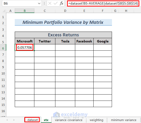
The formula uses the AVERAGE function to calculate the average of total stock returns Microsoft. Then it is subtracted from each stock return to get the Excess Return data. The dataset term in the formula means that the cell reference is coming from the dataset sheet.

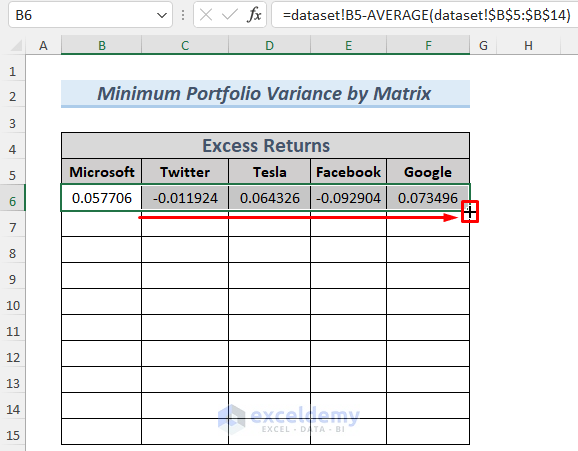
• Drag the Fill Handle to the right to AutoFill the cells to F6.

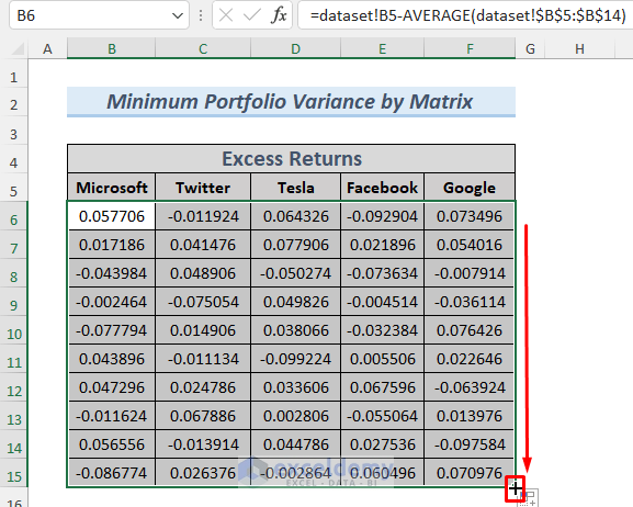
• Use the Fill Handle again to AutoFill all the cells. This command will return all the Excess Returns for 10 months.

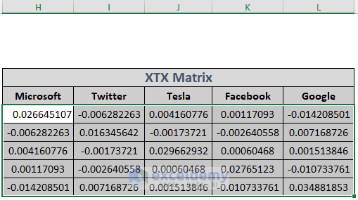
• Create a matrix by multiplying the transpose of the array B6:F15 with the B6:F15 We will use this matrix to determine the variance in the future. Create some columns to store the data of the matrix, select the 5×5 (multiplication between 5×10 and 10×5 matrices will result in a 5×5 matrix) range (H6:L10), and type the following formula in H6.

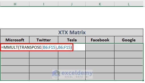
The formula uses the TRANSPOSE function to transpose the array B6:F15. The MMULT function returns the matrix multiplication result between this transposed array and B6:F15.

• Hold CTRL+SHIFT and press ENTER. Although it won’t give you any errors in the latest version of Excel, you get errors in the older version of Excel. You will see the output of the Matrix Multiplication in the sheet.

• Go to another new sheet for our convenience. Create necessary columns in it as well.
• Type the following formula in B5.

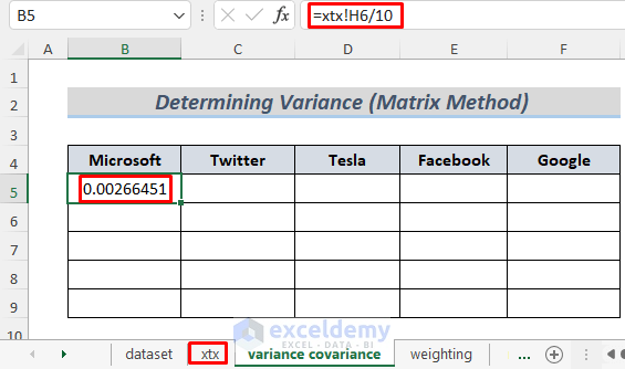
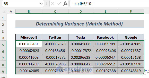
• Drag the Fill Icon to the right upto F5. Drag down the Fill Icon to AutoFill the lower cells. Create a Portfolio Return Matrix.

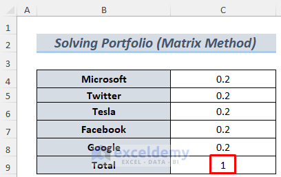
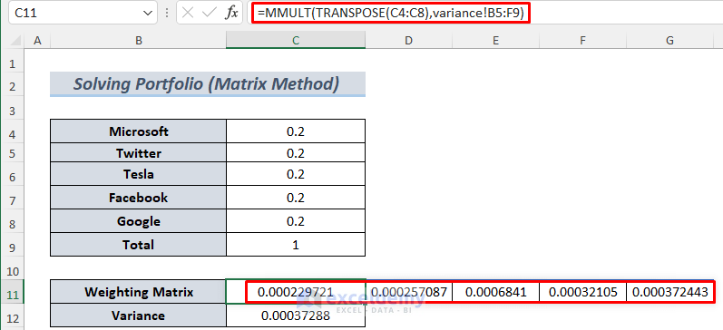
• Use some dummy data to solve our Portfolio. Select five decimal numbers that total to 1. If you have 6 companies, you should select 6 decimal numbers. We chose 2 as 0.2 times 5 equals 1. This is the hypothetical investment percentage for an investor.

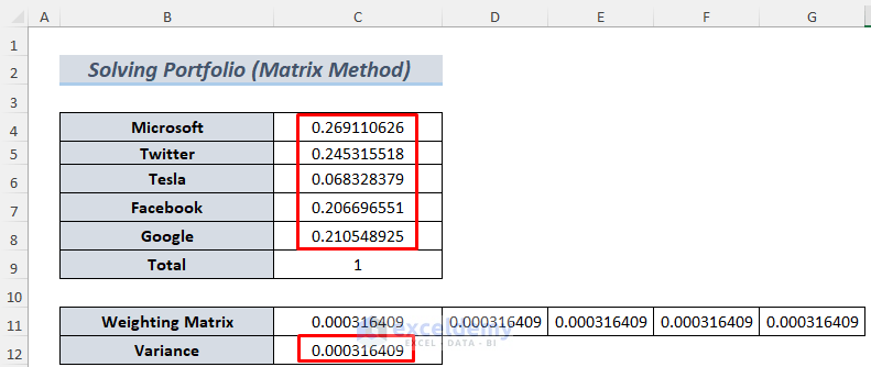
• Type the following formula in C11 to determine the Weighting Matrix. Make sure you select the array C11:G11 and hold CTRL+SHIFT before pressing ENTER. Although it won’t give you any errors in the latest version of Excel, you get errors in the older version.

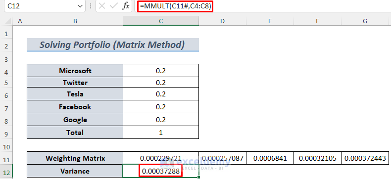
• Use the following formula to determine the Variance of our data.

• Need to use the Solver Toolpak to finish our job. If you don’t have this in your Data Tab, you need to go to the File Menu >> Options >> Add-ins >> Manage >> Excel Add-ins >> Go…

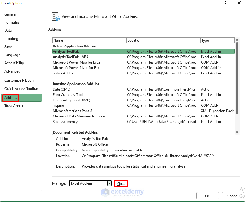
• The Add-ins window will appear. Check Solver Add-in and click OK.

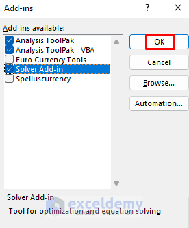
• The Solver Add-in will appear in the Data Tab. Click on it to open it.

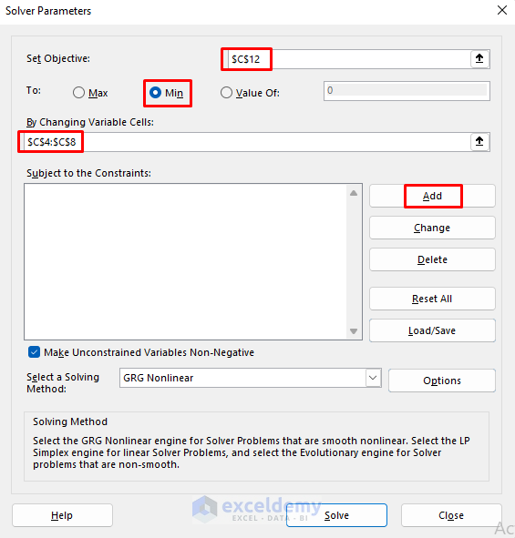
• Insert Solver Parameters. Here, we need to minimize the risk by minimizing the variance. So our Objective cell will be C12 which stores the value of Variance. Also, select Min.
• Select C4:C8 for Changing Variable Cells. Get the percentages of sustainable investment in these cells once we launch the Solver.
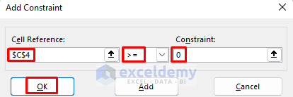
• Add some Constraints to get more accurate results.

• After clicking on Add, the Add Constraint dialog box will appear. Set the value of cell C4 to greater than or equal to zero.

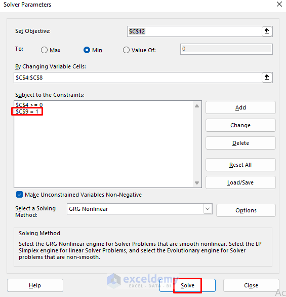
• We added another constraint which sets the value in C9 to 1.
• Click on Solve.

• The Solver Results window will appear. Click OK.

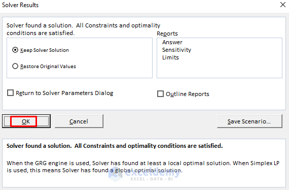
• You will see the minimized Variance and the risk-free investment percentage.

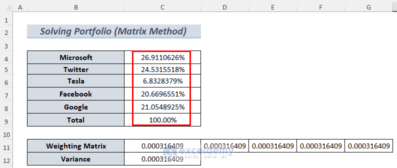
• Let’s convert these decimals to percentages. The output illustrates that 9110626% of investment in Microsoft, 24.5315518% of investment in Twitter, and so on will be risk-free for an investor.

Create a Minimum Variance Portfolio in Excel.

Method 2 – Minimum Variance Portfolio Comparing Two Assets

Steps:

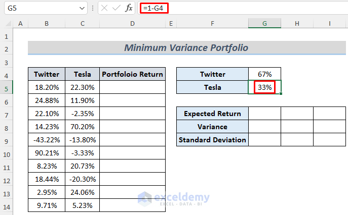
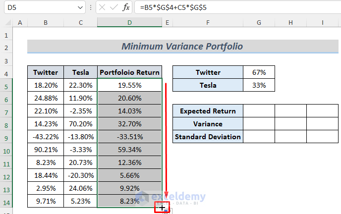
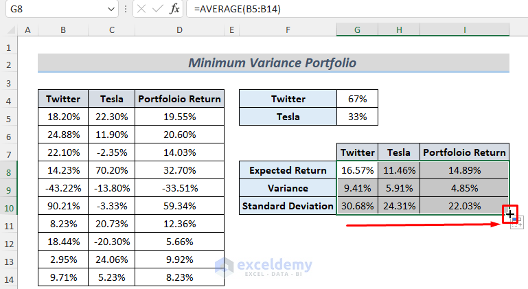
• Insert the stock return data and select some cells to store the necessary data, such as Standard Deviation or Variance. Set an initial investment percentage. We want to invest 67% in Twitter, and the rest in Tesla.
• Type the following formula in G5.

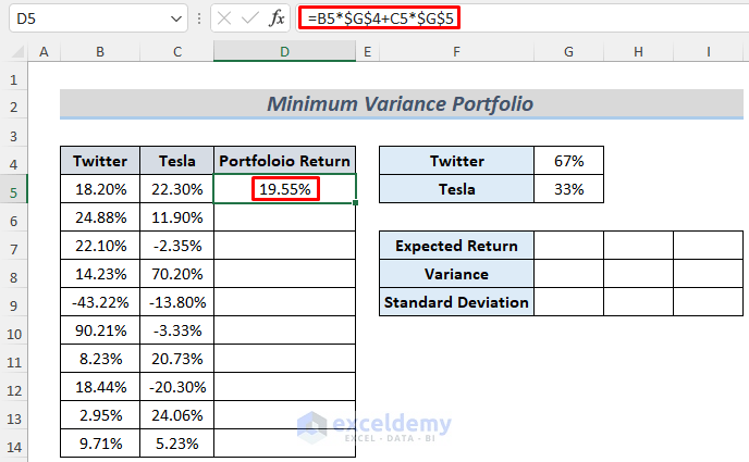
• Type the following formula in cell D5 which will return the Portfolio Return

• Use the Fill Handle to AutoFill the lower cells.

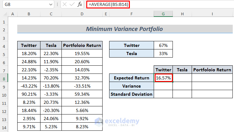
• Use another formula to calculate Expected Returns for Twitter, Tesla, and Portfolio Return.

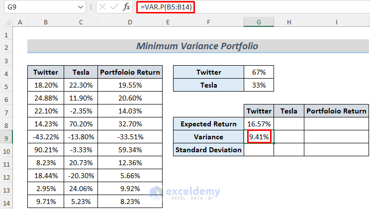
• Use the VAR.P function to calculate the variance of stock returns of Twitter. We want to ignore any logical values and text in the data, so we used the P function.

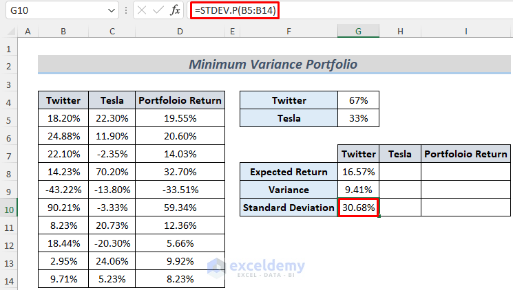
• Type the following formula to calculate Standard Deviation using the STDEV.P function.

• Drag the Fill Icon to the right to determine the Expected Return, Variance, and Standard Deviation for other data.

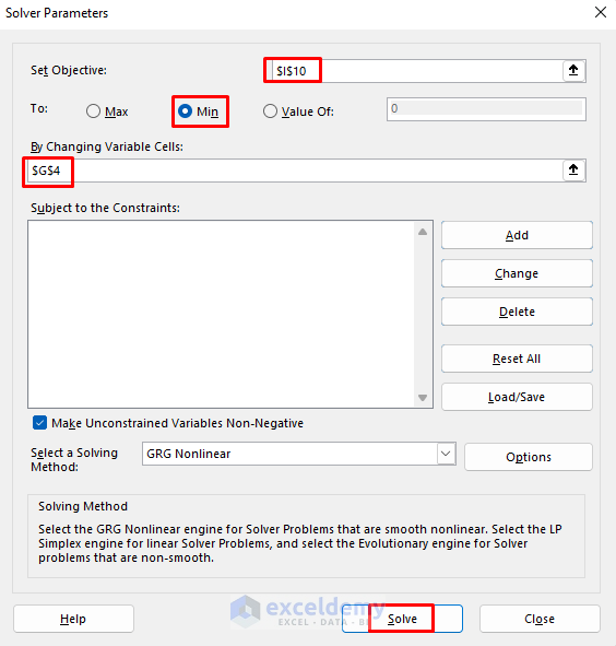
• Minimize the Variance or Standard Deviation (as Standard Deviation is simply the square root of Variance, we can use any of them for the Minimum Variance Portfolio).
• Insert the cell reference I10 where the Portfolio Return Standard Deviation is stored and set the Objective to Min.
• See the change by varying the investment percentage of Twitter. Insert the G4 cell reference in the ‘By Changing Variable Cells’ section.
• Cick Solve.

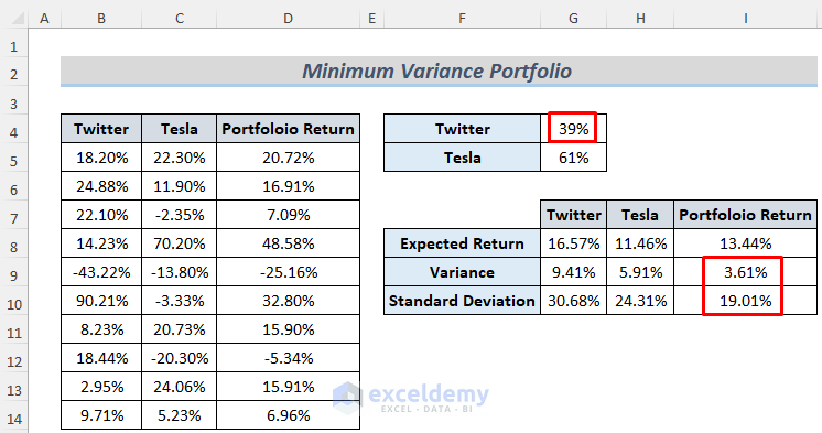
• Get the optimum value for the investment percentage in both Twitter and Tesla. Minimize the Variance from 85% to 3.61%.

Download Practice Workbook

Related Articles

• How to Calculate Variance Inflation Factor in Excel
• How to Calculate Semi Variance in Excel
• How to Calculate Schedule Variance Using Excel Formula
• How to Calculate Budget Variance in Excel
• How to Calculate Variance of Stock Returns in Excel
• How to Do Price Volume Variance Analysis in Excel

<< Go Back to Calculate Variance in Excel | Excel for Statistics | Learn Excel