In this article, we will demonstrate how to calculate Pooled Variance in Excel.
What Is Pooled Variance?
Pooled Variance is a statistical term also known as combined variance or composite variance. It indicates the average variance of two or more groups, and represents the single common variance among the groups.
Mathematically, Pooled Variance can be expressed as:
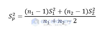
Where,
n1 = Sample size of Group 1,
n2 = Sample size of Group 2,
S12 = Variance of Group 1,
S22 = Variance of Group 2, and
Sp2 = Pooled Variance.
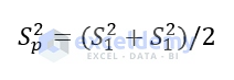
When the sample sizes are the same (n1=n2), we can use the following simplified formula:
How to Calculate Pooled Variance in Excel
Step 1 – Input Data and Form a Table
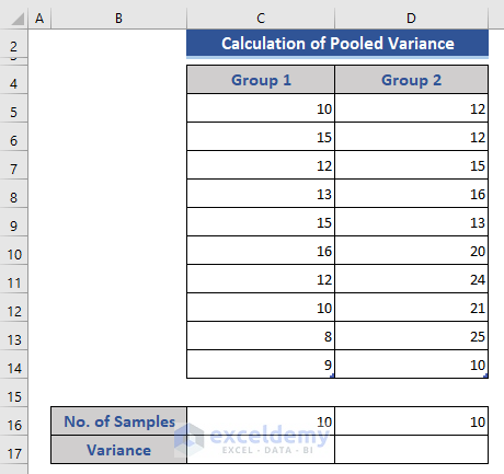
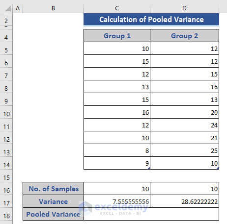
First, we collect sample data to make a dataset and form a Table, which will simplify our calculation.
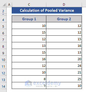
- Insert sample data from two different sources into the columns Group 1 and Group 2.
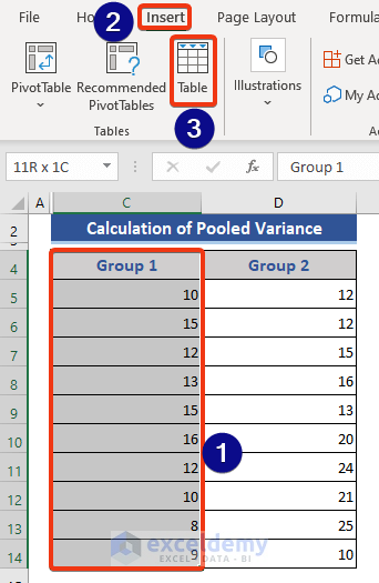
Now we form two tables from this data.
- Select the cells of the Group 1 column.
- Select Table from the Insert tab.
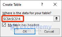
The Create Table window appears. Our selected range is pre-selected.
- Check My table has headers option.
- Click OK.
Click on the Table Design tab.
- Uncheck Filter Button and Banded Rows from the Table Style Options section.
- Set the name of the table in the Table Name field.
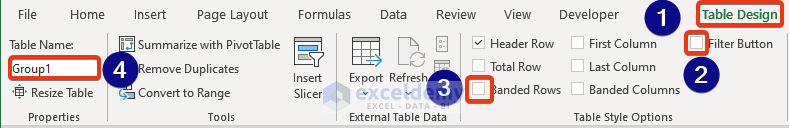
- Similarly, create the other table named Group2.
In the dataset, the little arrow in the bottom-right corner of the table denotes that it’s a Table. 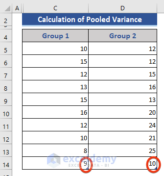
Read More: How to Do Variance Analysis in Excel
Step 2 – Count the Number of Samples
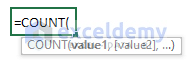
The COUNT function counts the number of cells in a range that contains numbers.
Using the 2 tables just created, we’ll now determine the size of the sample data using the COUNT function.
- Add a row to store the sample sizes.

- In cell C16, enter the following formula:
=COUNT(Group1)
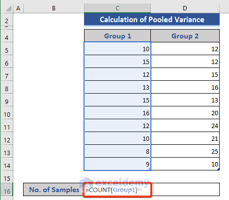
- Press Enter.
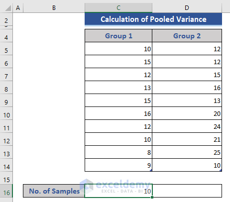
The data size of Group1 is returned.
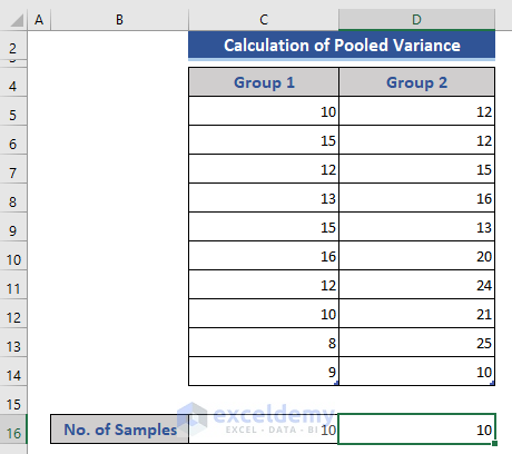
- Insert a similar formula for the Group2 table.
Read More: How to Apply Variance Formula in Excel to Get Plus-Minus Results
Step 3 – Calculate the Variance with the VAR.S Function
The VAR.S function estimates variance based on a sample (ignoring logical values and text in the sample).
With the sample sizes determined, we can determine the variance using Excel’s default variance function.
- Add a new row to store the variance figures.
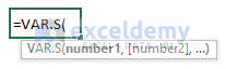
- In cell C17, enter the following formula:
=VAR.S(Group1)
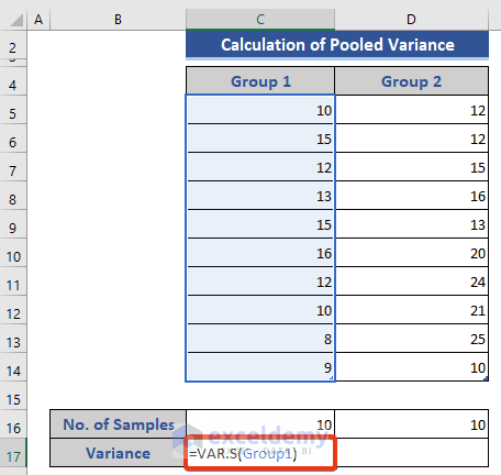
- Press Enter to return the result.
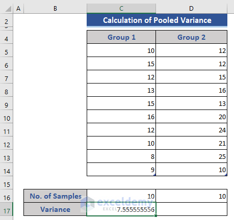
The variance for the data of the Group 1 column is returned.
- Create a similar formula for Group 2 in cell D17 and press Enter.
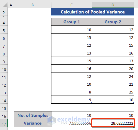
As we are using a Table as a reference, the Fill Handle will not work here.
Read More: How to Calculate Sample Variance in Excel
Step 4 – Determine Pooled Variance with a Formula
With the variances determined, we can calculate the Pooled Variance by applying a mathematical formula.
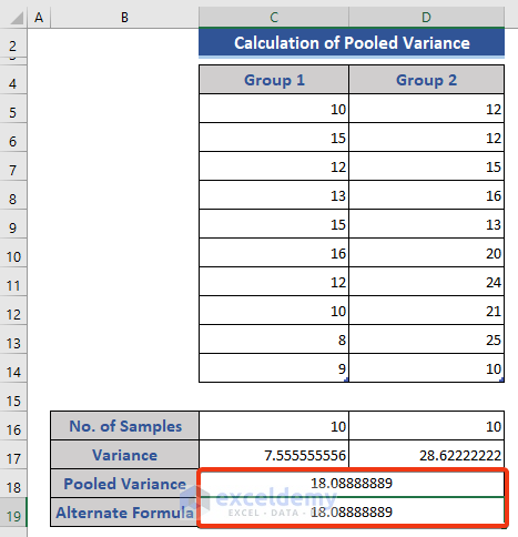
- Add a row for the Pooled Variance figures.
- Enter the following formula in cell C18:
=((C16-1)*C17+(D16-1)*D17)/(C16+D16-2)
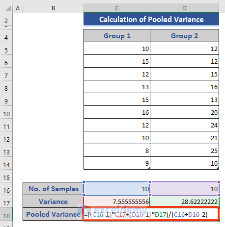
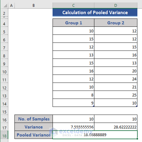
- Press Enter to return the result.
As discussed above, when the sample sizes are the same, we can use a simplified formula.
- Insert the following simplified formula in cell C19:
=(C17+D17)/2
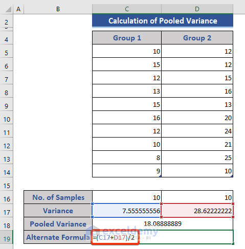
- Press Enter to return the result.
Read More: How to Calculate Percentage Variance between Two Numbers in Excel
Download Practice Workbook
Related Articles
- How to Calculate Coefficient of Variance in Excel
- How to Calculate Mean Variance and Standard Deviation in Excel
- How to Find Population Variance in Excel
- How to Find the Variance of a Probability Distribution in Excel
<< Go Back to Calculate Variance in Excel | Excel for Statistics | Learn Excel
Get FREE Advanced Excel Exercises with Solutions!
