If you are looking for how to use number with filter in Excel, then you are in the right place. In our practical life, we often need to filter our data and the numbering of the filtered data becomes distorted. Excel offers us various methods so that we can sort or filter our data with proper numbering. In this article, we’ll try to discuss how to number in Excel with filters.
How to Use Number in Excel with Filter: 5 Useful Methods
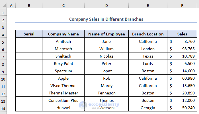
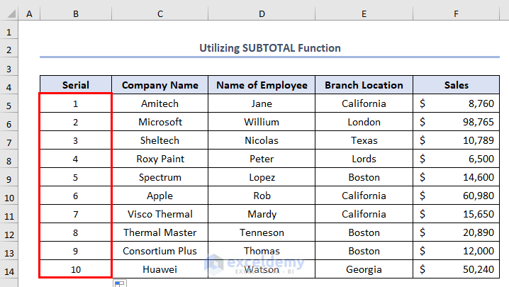
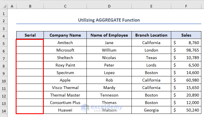
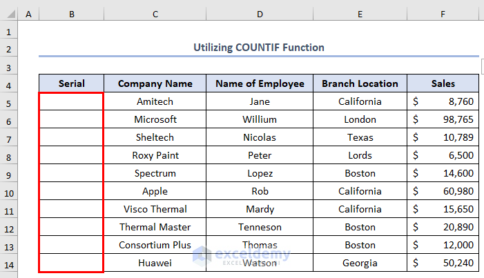
Excel offers various methods to number with filters. To show this we have made a dataset named Company Sales in Different Branches. It has column headers as Serial, Company Name, Name of Employee, Branch Location, and Sales. The dataset is like this.
Let’s see the methods to number in Excel with filters.
1. Utilizing SUBTOTAL Function to Use Number with Filter in Excel
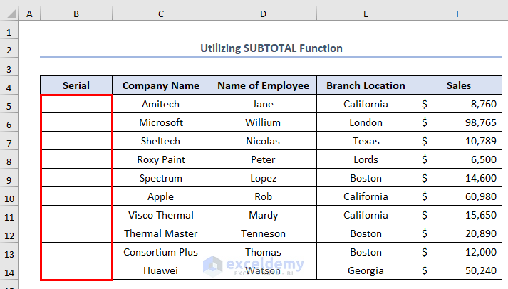
We can use the SUBTOTAL function when we need to add numbering as well as filter our desired data. We have to add numbers in the selected cells of the following picture. Another purpose of ours is to filter Amitech, Consortium, Spectrum, and Huawei from Company Name. Let’s follow the instructions below to use the SUBTOTAL formula in Excel for creating a serial number with filter.
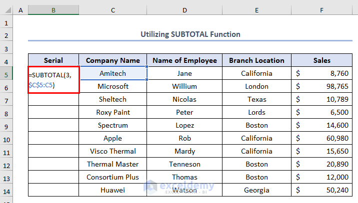
Firstly, write the following formula in the B5 cell.
=SUBTOTAL(3,$C$5:C5)Formula Breakdown
- $C$5:C5→ This denotes expanding range. The first element of the range i.e. $C$5 is locked, so the first element will always remain the same. The second element will change if we drag down the formula.
- Output → C5:C5
- 3,$C$5:C5 → 3 denotes the COUNTA function. In the picture below we have given a list of numbers that denote different functions in the case of the SUBTOTAL function.
- SUBTOTAL(3,$C$5:C5) → Gives us the total of cells with values in the selected range
- Output → 1
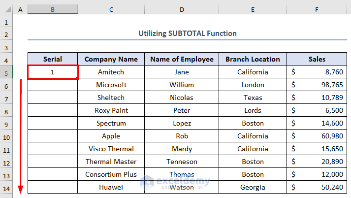
Secondly, press ENTER to get the output as 1.
Thirdly, use Fill Handle to get the other values in Cells B5:B14.
Consequently, we’ll get the output like this as added numbers in the B Column.
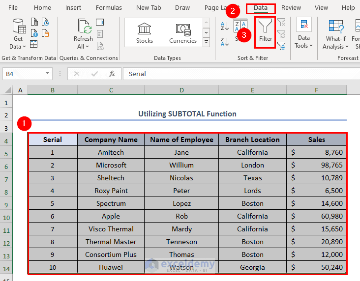
Fourthly, to filter the required Company Names, select the whole dataset > go to Data > click Filter.
As a result, we’ll have the filter icons in every Column Header.
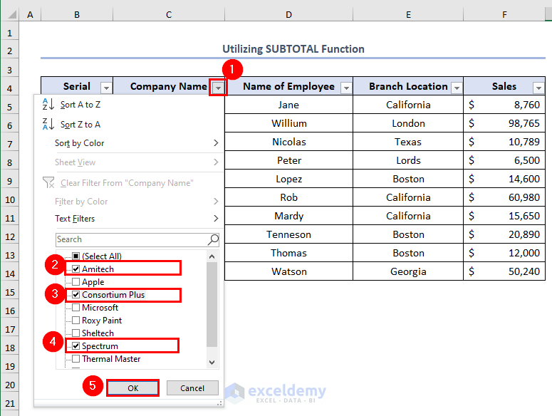
Fifthly, select the icon in the Company Name column header > select Amitech, Consortium Plus, Spectrum > click OK.
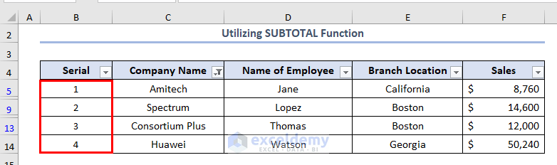
Eventually, we’ll get the output like this where specified Company Names are filtered and Serial Numbers in a chronological way.
2. Using AGGREGATE Function
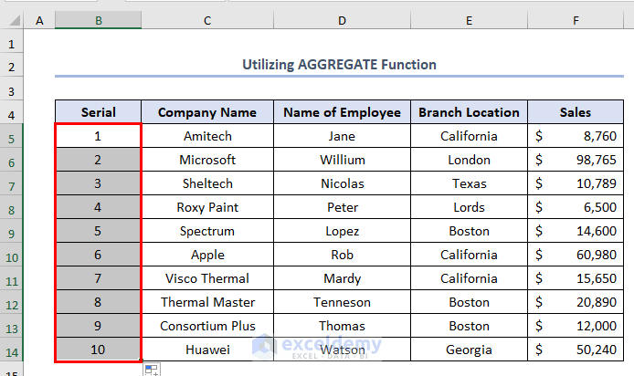
The objective of usage of the AGGREGATE function is the same as the SUBTOTAL function with different strings. We need to add numbers in the selected cells and filter Jane, Nicolas, and Thomas from the Name of Employee column.
Firstly, write the following formula in the B5 cell.
=AGGREGATE(3,7,$D$5:D5)Formula Breakdown
- $D$5:D5 → Denotes the expandable range
- 3 → Activates the COUNTA function
- 7 → Denotes Ignore Hidden Rows and Error Values
- AGGREGATE(3,7,$D$5:D5) → Denotes the sum of the COUNTA excluding hidden rows and error values

Secondly, press ENTER and use Fill Handle to get the output of numbers in a chronological manner.
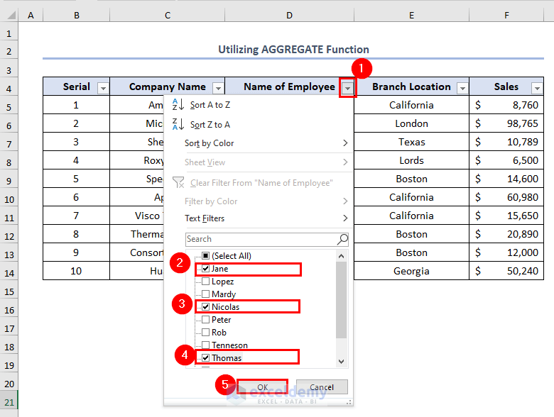
Thirdly, to filter the Name of Employee create a filter option in the Column Headers as we have done before.
Fourthly, click the filter icon in the column of Name of Employee > select Jane, Nicolas, Thomas > click OK.
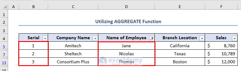
As a result, we’ll get an output like this where specified names are filtered and numbers are added in a chronological manner.
Read More: How to Create a Number Sequence in Excel Based on Criteria
3. Applying ROW Function to Use Number with Filter in Excel
We can add the ROW function to the number in Excel. We need to number the following selected cells and will try to filter California from the Branch Location column.
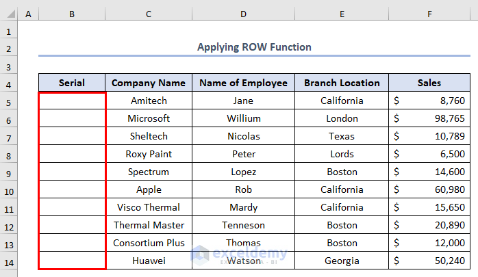
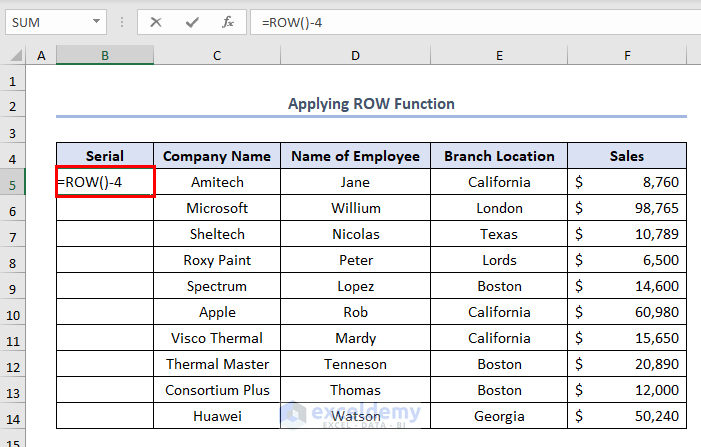
To do this, firstly, write the following formula in the B5 cell.
=ROW()-4Formula Breakdown
- ROW() → Denotes the number of rows (Here, it is B5 Cell)
- Output → 5
- ROW()-4 → Denotes the number after subtracting 4
- Explanation → 5-4 =1
- Output → 1
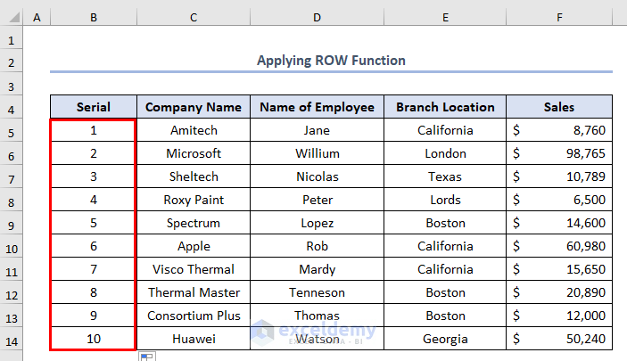
Similarly, as before, press ENTER and use Fill Handle to get numbers in the Serial column.
Thirdly, to filter California, select the filter mark in the Branch Location column > select California > click OK.
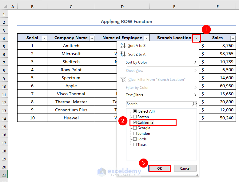
Eventually, we’ll get the output like this.
Here, we can see that the numbers in the B Column are not sorted chronologically.

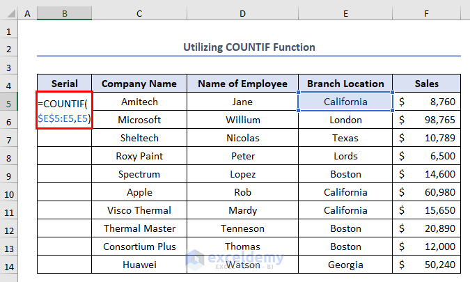
4. Using COUNTIF Function
The COUNTIF function is another function to number with filters. We need to add numbers in the B Column and filter California from Branch Location.
Firstly, write the following formula in the B5 cell.
=COUNTIF($E$5:E5,E5)Formula Breakdown
- $E$5:E5 → Denotes the expandable range
- E5) → Denotes the value in the D5 cell
- Output → California
- COUNTIF($E$5:E5, E5) →The COUNTIF function counts the number of cells with the value of D5 cell.
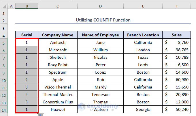
Secondly, press ENTER and use Fill Handle and get the output like this.
Importantly, we can see that the numbers are not sorted chronologically. But it will be chronological when we’ll filter our required place.
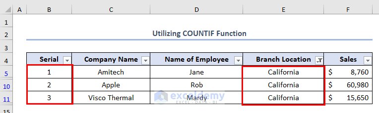
Thirdly, select the filter mark in the Branch Location column > click California > click OK.

Eventually, we’ll find our output like this where the numbers are no more unsorted and filtration of California has been done.
Read More: How to Add Automatic Serial Number with Formula in Excel
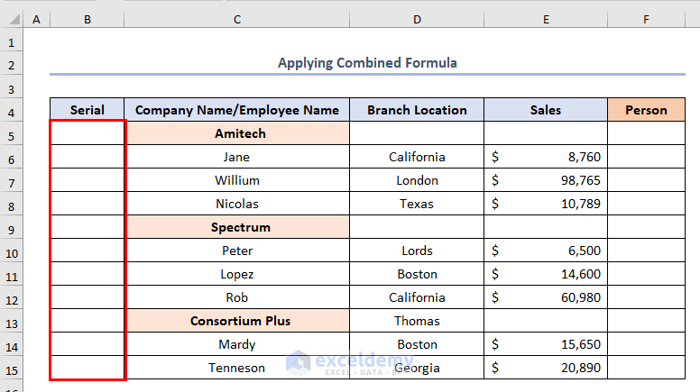
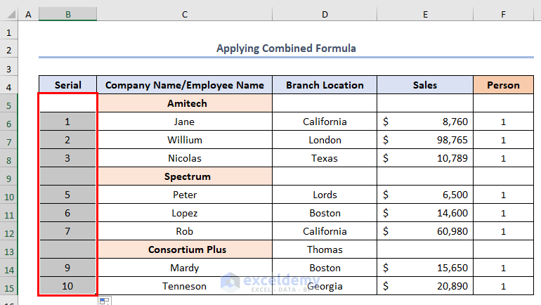
5. Utilizing Combined Formula
We can use the combination of IF, LEFT, and SUBTOTAL functions to number Excel Rows. We have made the following dataset to number the marked Rows.
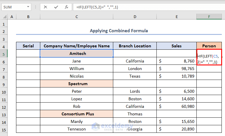
Firstly, we’ll use the combination of IF and LEFT functions to be sure that the entities are a person or not. After this surety, we’ll apply the SUBTOTAL function to the output.
In this case, we will first determine whether the Company Name/Employee Name column entries are of people or not. There are two spaces in the sheet before the name of each department. As a result, any non-name entry will have two spaces on the left. Using this condition, we can determine whether the entry is a person’s name or not.
Eventually, write the formula in the F5 cell like this.
=IF(LEFT(C5,2)=” “,””,1)Formula Breakdown
- LEFT(C5,2) → Fetches two characters from the left of cell C5.
- Output → Double space
- LEFT(C5,2)=” ” →This logical test denotes whether the left two characters of cell C5 are two spaces or not.
- Output → TRUE
- Explanation → The left two characters is equal to double spaces.
- IF(LEFT(C5,2)=” “,””,1) → The IF function returns a blank if the above condition is satisfied. Otherwise, it returns the value
- Output → Blank
- Explanation → In this case the left two characters are double space.
- Output → Blank
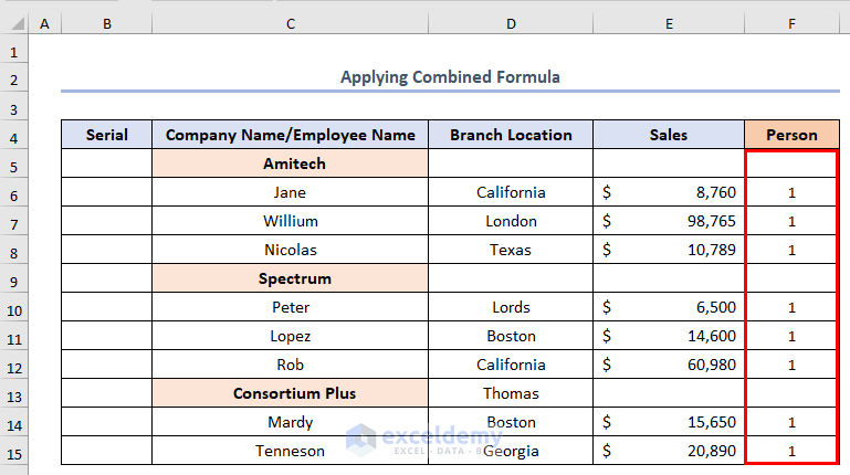
After pressing ENTER and using Fill Handle, we’ll get the output like this.
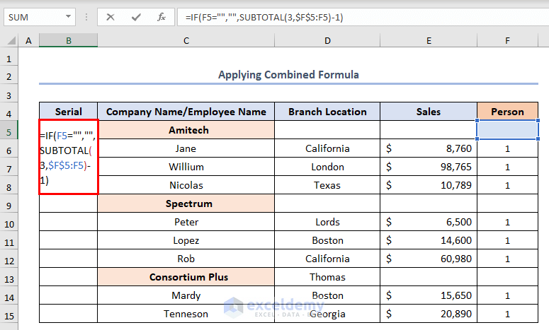
After determining whether the name is an employee or not, we’ll add numbers easily in the B Column by writing the following formula.
=IF(F5=””,””,SUBTOTAL(3,$F$5:F5)-1)Formula Breakdown
F5=”” → Determines whether the value in the F6 cell is blank.
Output → TRUE
Explanation → F5 cell is blank.
SUBTOTAL(3,$F$5:F5)-1 → Returns value of the expandable range $F$5:F5 as shown in method 2.
IF(F5=””,””,SUBTOTAL(3,$F$5:F5)-1) → The IF function returns the value blank if the above condition is satisfied. It gives the value of SUBTOTAL(3,$F$5:F5)-1 if the corresponding cell is in Person the column is not blank.
Output → Blank
Explanation → F5 cell is blank.
Eventually, pressing ENTER and using Fill Handle we find the following output.
Things to Remember
- We can use the Row function to number Rows This function is not related to filtering. That’s why after filtering, we can see from Method 4 that numbering is no more in a chronological manner. Because the ROW function doesn’t have any string which will detect the hidden or unused Rows like the SUBTOTAL, AGGREGATE, or COUNTIF functions do. So, the ROW function is not the best option when we need both numbering and filtering.
- We can use the Combined formula to number individual types such as numbering the names in Amitech or Spectrum or Consortium Plus.For example, in the case of Spectrum type, we just need to change the formula from IF(F10=””,””,SUBTOTAL(3,$F$5:F10)-1) to IF(F10=””,””,SUBTOTAL(3,$F$9:F10)-1).
Download Practice Workbook
Conclusion
We can number Excel Rows as well as filter effectively if we study this article properly. Please feel free to comment any queries or suggestions down below.
Related Articles
- How to Perform Numbering in One Cell in Excel
- How to Add Numbers 1 2 3 in Excel
- How to Create a Number Sequence with Text in Excel
- How to Create a Number Sequence in Excel Without Dragging
- How to Increment Row Number in Excel Formula
<< Go Back to Serial Number in Excel | Numbering in Excel | Learn Excel
Get FREE Advanced Excel Exercises with Solutions!
