Subtotal Formula in Excel for Serial Number: 3 Suitable Methods

Method 1 – Use of SUBTOTAL Function for Serial Number

Steps:

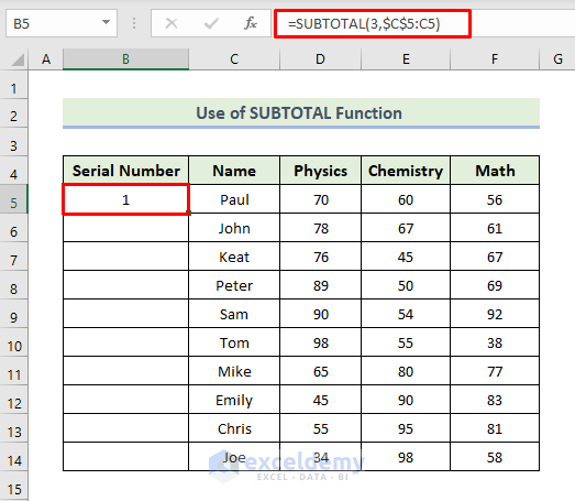
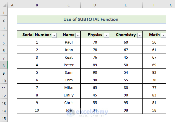
Select Cell B5 and type the formula below.

=SUBTOTAL(3,$C$5:C5)

Press Enter.

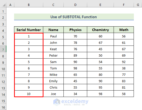
Subtotal Formula in Excel for Serial Number

Drag the Fill Handle icon to fill the other cells with the above formula.
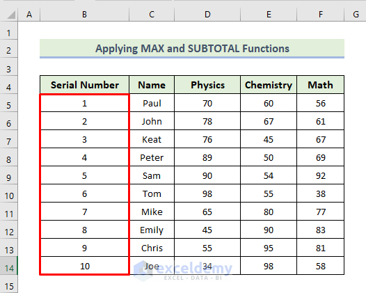
Get the following serial number.

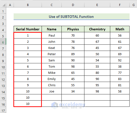
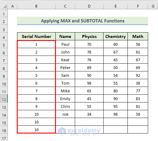
See that no new serial is created for the cells with no corresponding values for the related cells if we drag the Fill Handle icon into the next few cells.

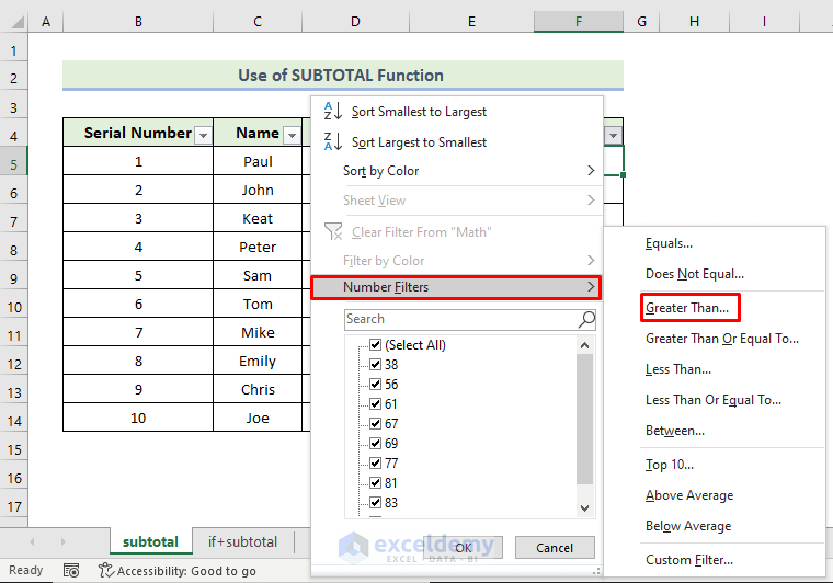
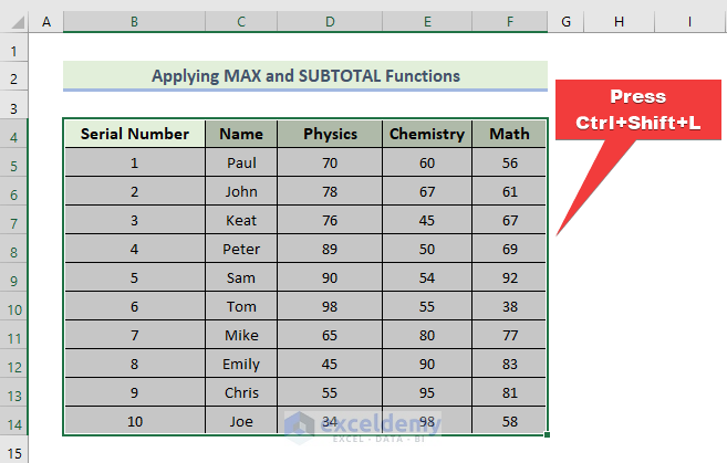
Filter the data to show the only visible column serial number in the dataset.
Select the range of cells and press Ctrl+Shift+L.

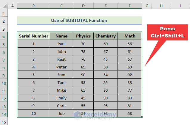
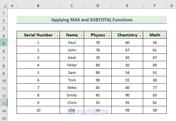
Add a filter to the data, as shown below.

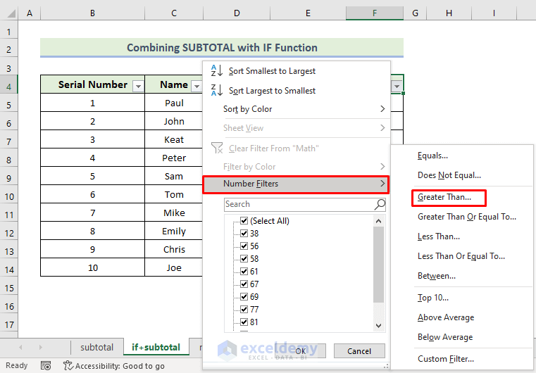
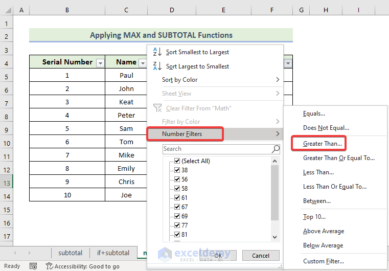
Click on the Math column drop-down icon, select Number Filters, and finally select Greater Than option.

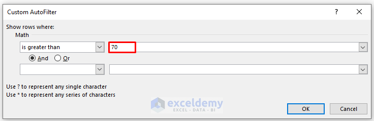
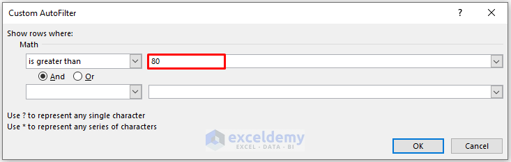
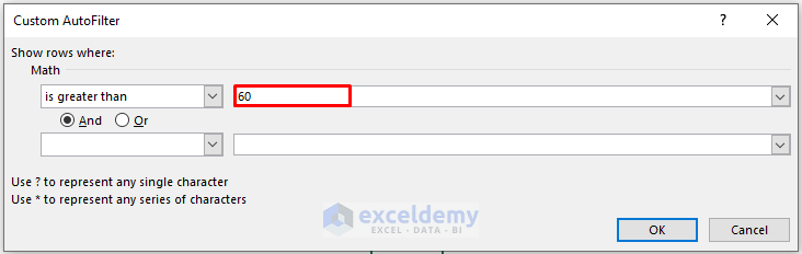
The Custom AutoFilter window appears, type your required number in the is greater than a box.
Click OK.

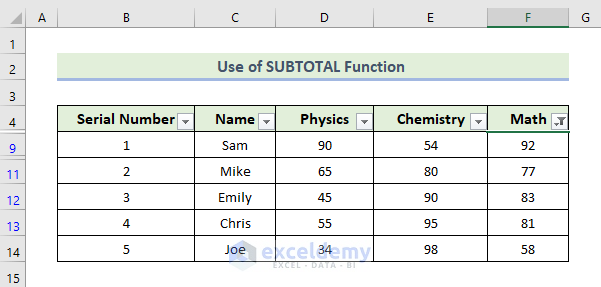
Filter the Math column data based on a score greater than 70, you will get the following column. The serial number is automatically generated when the column is reduced according to the criteria.

Method 2 – Combining SUBTOTAL with IF Function

Steps:

Select Cell B5 and type the formula below.

=IF(C5="","",SUBTOTAL(3,$C$5:C5))

Press Enter.

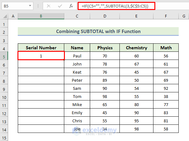
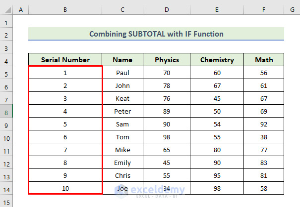
Drag the Fill Handle icon to fill the other cells with the above formula.
Get the following serial number.

Filter the data to show the only column serial number in the dataset.
Select the range of cells and press Ctrl+Shift+L.

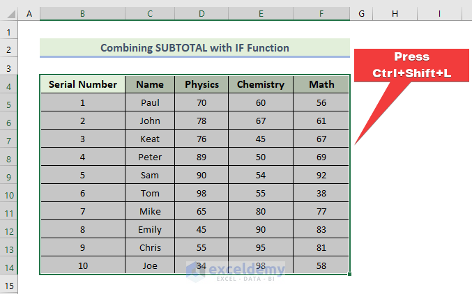
Add a filter to the data, as shown below.

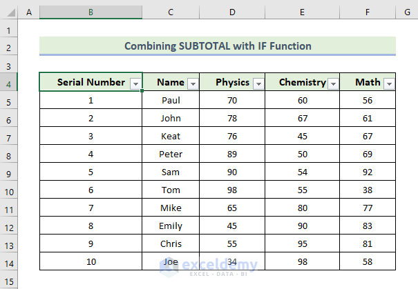
Click on the Math column drop-down icon, select Number Filters, and finally select Greater Than option.

The Custom AutoFilter window appears, type your required number in the is greater than box.
Click OK.

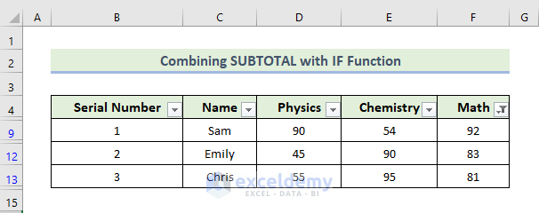
Filter the Math column data based on a score greater than 80. The serial number is automatically generated when the column is reduced according to the criteria.

How Does the Formula Work?

SUBTOTAL(3,$C$5:C5)

In this formula, we have used the SUBTOTAL function. The first argument indicates the function number. And function number 3 refers to the COUNTA functions. It will count the cells in the range $C$5:C5.

IF(C5=””,””,SUBTOTAL(3,$C$5:C5))

If Cell C5 is empty, the IF function will return blank; otherwise, it will return the SUBTOTAL function value.

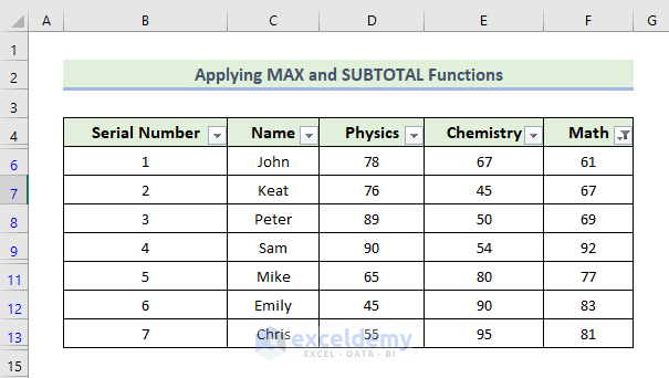
Method 3 – Applying MAX and SUBTOTAL Functions

Steps:

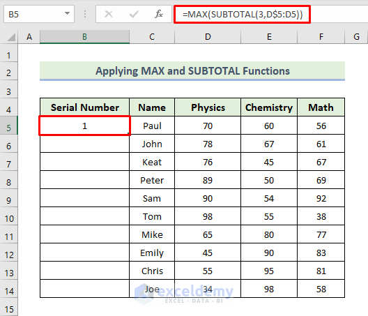
Select Cell B5 and type the formula below.

=MAX(SUBTOTAL(3,D$5:D5))

Press Enter.

Drag the Fill Handle icon to fill the other cells with the above formula.
Get the following serial number.

No new serial is created for the cells where there are no corresponding values for the related cells if we drag the Fill Handle icon into the next few cells.

Filter the data to show the only column serial number in the dataset.
Select the range of cells and press Ctrl+Shift+L.

Add a filter to the data, as shown below.

Click on the Math column drop-down icon, select Number Filters, and finally select Greater Than option.

When the Custom AutoFilter window appears, type your required number in the is greater than box.
Click OK.

Get the following column when you filter the Math column data based on a score greater than 70. The serial number is automatically generated when the column is reduced according to the criteria.

How Does the Formula Work?

SUBTOTAL(3,$C$5:C5)

We used the SUBTOTAL function. The first argument indicates the function number. And function number 3 refers to the COUNTA function. Count the cells in the range $C$5:C5.

MAX(SUBTOTAL(3,D$5:D5))

The MAX function will return the largest value in the list of arguments.

Things to Remember

When you are creating serial numbers using the subtotal formula, you need to keep certain things in mind.

✎ You should keep in mind that Excel doesn’t consider hidden values the same as the filtered-out values. So, when you hide any rows the serial will not generate automatically.

✎ When using multiple functions in one formula, you need to put the parenthesis carefully, otherwise, the formula will not be executed.

Download Practice Workbook

Download this practice workbook to exercise while you are reading this article. It contains all the datasets in different spreadsheets for a clear understanding. Try yourself while you go through the step-by-step process.

Subtotal Formula for Serial Number.xlsx